As a data scientist, one often encounters dependent variables that are proportions: for example, the number of successes divided by the number of attempts, party vote, proportion of money spent for something, or the attendance rate of public events. Modeling and predicting such variables in a regression framework is possible, but one has to go beyond the standard linear model, because the data are restricted to the range between 0 and 1. Popular logistic regression is not suitable either, because it permits only 0s and 1s, but not an attendance rate of .80 or 80 %. In this blog post, I will compare different models that are available for proportions and illustrate them to predict the attendance rate of matches of the German Handball-Bundesliga.
Modeling Proportion Data
As a starting point, a linear regression model without a link function may be considered to get one started. The model is obviously wrong, because it will easily make predictions smaller than 0 or larger than 1. Nevertheless, it may work okay especially for intermediate proportions.
A second option is a binomial or quasi-binomial model. Therein, the proportion is conceived of as the outcome of multiple binomial trials. A good example are the shots of a basketball player, where one may either model each individual shot using a logistic model for outcomes of 0 and 1. Or one may aggregate all attempts in a match and model the proportion of successful shots, which is a value in the interval of [0, 1], using a (quasi-)binomial model.
A related option is a Poisson model for count data that, for example, may be used to model the number of occurrences of a specific symptom per week or month. However, the model is not quite the right choice if the count variable may take on values of several thousand spectators of a sport event. More importantly, it can fail to capture, for example, the difference between 1,000 spectators in a stadium with a capacity of 1,000 (i.e., 100 %) and 2,000 spectators in a stadium of 5,000 (i.e., 40 %).
The third option considered is beta regression which assumes that the dependent variable is beta-distributed. This model is very flexible and ideally suited for original proportions or rates. However, it should be noted that it assumes values in the interval (0, 1), that is, 0 and 1 are excluded. There are two variants of beta regression: One predicts only the mean of the dependent variable whereas the second variant models also the dispersion parameter phi. This sounds attractive for the current problem, because handball teams like Flensburg almost always have attendance rates of over 90 % (small variance) while the attendance rates in other stadiums may show more variability.
Application: Handball-Bundesliga
Data from the German Handball-Bundesliga were obtained for the current and the last two seasons from https://www.dkb-handball-bundesliga.de. The data needed some wrangling and cleansing and are not perfectly valid (e.g., some entries exhibit attendance rate larger than 100 %), but will suffice for the present purpose. You can find the respective R code on my Github.
Setup
library("conflicted")
suppressPackageStartupMessages(library("tidyverse"))
conflict_prefer("filter", "dplyr")
#> [conflicted] Will prefer dplyr::filter over any other package
library("betareg")
library("broom")
library("kableExtra")
theme_set(theme_light(base_size = 12))
theme_update(panel.grid.minor = element_blank())

# Function to transform attendance rates for beta regression because values of 0
# and/or 1 may occur
transform_perc <- function(percentage_vec) {
    # See Cribari-Neto & Zeileis (2010)
    (percentage_vec * (length(percentage_vec) - 1) + 0.5)/length(percentage_vec)
}
Selected Variables
Dependent variable:
- Beta regression: Attendance rate; values were transformed to the interval (0, 1) using
transform_perc() - Quasi-binomial regression: Attendance rate in the interval [0, 1]
- Linear regression: Attendance (i.e., count)
- In all cases, entries where the attendance was larger than the capacity were replaced with the maximum capacity.
Independent variables:
- Home team: Different teams have different average attendance rates and/or stadium capacities. For the beta model, home team was also used to predict the dispersion parameter phi.
- Away team: Generally, more successful away teams like Kiel attract more spectators.
- Year/season: Used to capture potential differences across the three seasons.
- Weekday: Matches on weekends probably attract more spectators.
- All variables are categorical variables and appropriate coding schemes (i.e., dummy or effect coding where chosen).
Initial Results for Beta Regression
# Use data from 2016/17 and 2017/18
df21 <- filter(df1, season_id != 55149) %>%
    mutate(year = droplevels(year),
           home_team = droplevels(home_team),
           away_team = droplevels(away_team)) %>%
    mutate(y = transform_perc(perc))

# Use effect coding, contr.sum(), for teams so that intercept corresponds to
# average across all teams
contrasts(df21$home_team) <- contr.sum(levels(df21$home_team))
colnames(contrasts(df21$home_team)) <- head(levels(df21$home_team), -1)
contrasts(df21$away_team) <- contr.sum(levels(df21$away_team))
colnames(contrasts(df21$away_team)) <- head(levels(df21$away_team), -1)

# Dummy coding
contrasts(df21$weekday) <- contr.treatment(7, base = 6)
The first model I want to show is a beta regression model.
As you can see below, the intercept is equal to 2.08 on the logit scale.
Thus, the model predicts an average attendance rate of 89 % (plogis(2.08)).
Average here means averaged across all teams (since effect coding was used) and predicted for a match on Saturday in the season 2016/17 (dummy coding used for weekday and year).
Furthermore, there are huge differences across teams.
For example, the predicted value for a home match of Flensburg is 2.08 + 1.42 corresponding to an attendance rate of 97 % (plogis(3.5)) but only 84 % (plogis(2.08 - 0.42)) for Lemgo or 63 % for Lübbecke.
Likewise, the attendance rate differs by away team, where, for example, matches against Kiel are more attractive than matches against Erlangen.
Apart from that, the precision or variability of the predicted mean also varies as a function of home team. For example, the precision is larger (and variability lower) for Flensburg than for Lemgo.
m1 <- betareg(y ~ home_team + away_team + weekday + year
              | home_team, data = df21)
m1_est <- tidy(m1)

# Print some estimates
slice(m1_est, 1, 49, seq(2, 69, 8))
#> # A tibble: 11 x 6
#>    component term                    estimate std.error statistic   p.value
#>    <chr>     <chr>                      <dbl>     <dbl>     <dbl>     <dbl>
#>  1 mean      (Intercept)               2.08      0.0815    25.5   2.54e-143
#>  2 precision (Intercept)               2.40      0.0643    37.4   2.44e-305
#>  3 mean      home_teamSG Flensburg-~   1.42      0.193      7.39  1.48e- 13
#>  4 mean      home_teamTBV Lemgo Lip~  -0.422     0.125     -3.38  7.23e-  4
#>  5 mean      home_teamTuS N-Lübbecke  -1.53      0.168     -9.08  1.07e- 19
#>  6 mean      away_teamTHW Kiel         0.728     0.123      5.94  2.78e-  9
#>  7 mean      away_teamHC Erlangen     -0.161     0.119     -1.35  1.77e-  1
#>  8 mean      weekday1                  0.291     0.257      1.13  2.57e-  1
#>  9 precision home_teamSG Flensburg-~   0.491     0.270      1.82  6.85e-  2
#> 10 precision home_teamTBV Lemgo Lip~   0.0346    0.235      0.147 8.83e-  1
#> 11 precision home_teamTuS N-Lübbecke  -0.374     0.313     -1.19  2.32e-  1
Illustrative Plot of Estimates
The model estimates can also be illustrated graphically.
The parameters mean (mu) and precision (phi) from above correspond to a beta distribution, which is specific to each home team in the fitted model.
To calculate the densities of the beta distribution using dbeta(), I first have to transform the estimates from the model.
# Function to calculate a and b parameter of beta distribution from mu and phi
# used in betareg with link function logit for mu and log for phi
calc_ab <- function(mu, phi) {
    mu <- plogis(mu)
    phi <- exp(phi)
    b <- phi - mu*phi
    a <- phi - b
    return(cbind(a = a, b = b)[, 1:2])
}

# Calculate predicted beta distributions for Flensburg and Lemgo
preds1 <-
    # Estimates of mu and phi from above
    calc_ab(2.08 + c(1.42, -.42), 2.4 + c(.49, .03)) %>%
    asplit(1) %>%
    setNames(c("SG Flensburg-Handewitt", "TBV Lemgo Lippe")) %>%
    # Calculate densities via dbeta()
    lapply(function(y) data.frame(x = seq(0, 1, .001),
                                  y = dbeta(seq(0, 1, .001), y[1], y[2]))) %>%
    enframe("home_team") %>%
    unnest(value)

# Print some values
slice(preds1, seq(701, by = 100, length.out = 4))
#> # A tibble: 4 x 3
#>   home_team                  x        y
#>   <chr>                  <dbl>    <dbl>
#> 1 SG Flensburg-Handewitt   0.7   0.0133
#> 2 SG Flensburg-Handewitt   0.8   0.145
#> 3 SG Flensburg-Handewitt   0.9   1.40
#> 4 SG Flensburg-Handewitt   1   Inf
Below, I plotted the model-implied beta distributions for the two teams, which are illustrated using the green lines.
Furthermore, the plot shows the predicted means (green point on the x-axis), the raw densities calculated by geom_density() across the 34 matches per team, as well as the observed attendance rate for each match (placed below the densities by geom_rug()).
In summary, the plot nicely illustrates the estimates from above, namely, very high and homogeneous attendance rates for Flensburg and lower and more varied attendance rates for Lemgo. This aligns quite well with the observed data. Note also that I picked these two teams more or less at random, but estimates are of course available for all teams in the data set.
# Plot observed data using densities and rugs
p1 <- df21 %>%
    filter(home_team %in% c("SG Flensburg-Handewitt", "TBV Lemgo Lippe")) %>%
    ggplot(aes(x = perc, fill = home_team)) +
    geom_density(trim = TRUE) +
    geom_rug() +
    facet_wrap(~ home_team) +
    coord_cartesian(xlim = c(.5, 1), ylim = c(0, 12)) +
    scale_fill_viridis_d() +
    labs(y = "Density", x = "Attendance Rate", fill = NULL,
         title = "Beta Regression: Observed and Fitted Attendance Rates") +
    theme(legend.position = "none")

# Add lines corresponding to estimated distributions
p1 <- p1 +
    geom_line(data = preds1, aes(x = x, y = y),
              inherit.aes = FALSE, size = 1,
              color = rgb(0, 155, 149, maxColorValue = 255))

# Add predicted means
p1 <- p1 +
    geom_point(data = data.frame(y = 0,
                                 x = plogis(2.01 + c(1.49, -.35)),
                                 home_team = c("SG Flensburg-Handewitt", "TBV Lemgo Lippe")),
               aes(x = x, y = y), show.legend = FALSE, size = 3,
               color = rgb(0, 155, 149, maxColorValue = 255))
p1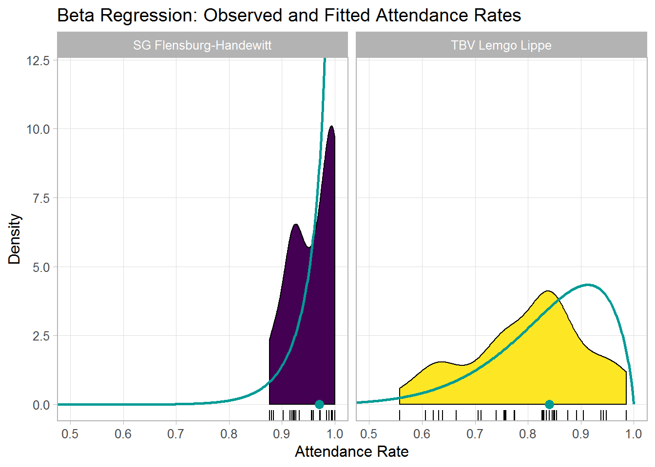
Residuals
Finally, I want to have a quick look at the residuals (which are on the logit scale). I decided to plot them chronologically, that is, against match day. As you see, residuals tend to get higher across the course of a season indicating that attendance rates near the end of the season are slightly higher than predicted. Thus, it seems useful to add variables to the model that can capture this effect (see below).
m1_res <- augment(m1, data = df21)

ggplot(m1_res, aes(x = round_number, y = .resid)) +
        geom_point() +
        stat_smooth(method = "loess", formula = "y ~ x") +
        facet_wrap(~ year) +
        labs(y = "Residuals", x = "Match Day",
             title = "Residuals as a Function of Match Day")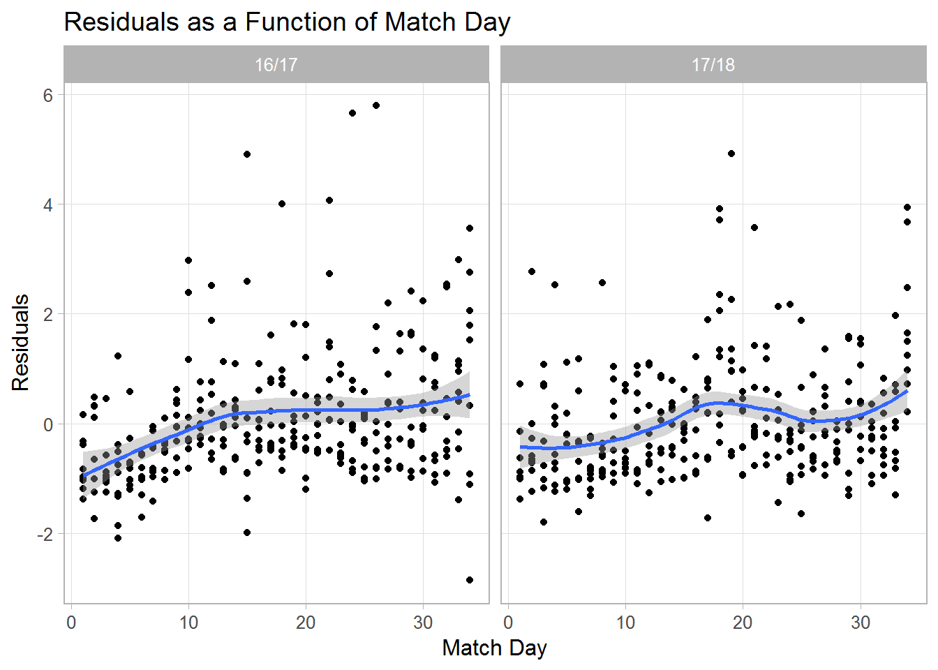
Model Comparisons
Models Considered
In the following, I will compare different models:
- The models will either model the variable matchday using a linear trend. Or the trend over time will be captured by the categorical variable month (thus allowing different attendance rates in each month). More information about the coding for variable month is provided in part 2.
- Furthermore, I will compare different different link functions or forms:
- Linear model (lm)
- Quasi-binomial model (binomial)
- Beta regression (beta)
- Beta regression with dispersion parameter and logit link (beta+ logit)
- Beta regression with dispersion parameter and loglog link (beta+ loglog)
The performance of the models will be evaluated relative to the training data set from above (season 2016/17 and 2017/18) and to a holdout or cross-validation data set (season 2018/19). Furthermore, I will compare the models relative to simply predicting the average attendance rate of the home team.
res11 <- list()

### Average ###

# This "model" simply predicts for each match the yearly average attendance rate
# of the home team
res11$average_no <-
  glm(perc ~ home_team*year, data = df21,
        family = quasibinomial(logit), weights = capacity)

### beta+dispersion (logit) ###

res11$betaDsplogit_lin <-
    betareg(y ~ home_team + away_team + weekday + year + half2 +
                matchday | home_team, data = df21)
res11$betaDsplogit_mon <-
    betareg(y ~ home_team + away_team + weekday + year + half2 +
                Oct + Nov + Dec + Mar + Apr + May | home_team, data = df21)

### beta+dispersion (loglog) ###

res11$betaDsploglog_lin <-
    update(res11$betaDsplogit_lin, link = "loglog")
res11$betaDsploglog_mon <-
    update(res11$betaDsplogit_mon, link = "loglog")

### beta (logit) ###

res11$beta_lin <-
    betareg(y ~ home_team + away_team + weekday + year + half2 +
                matchday, data = df21)
res11$beta_mon <-
    betareg(y ~ home_team + away_team + weekday + year + half2 +
                Oct + Nov + Dec + Mar + Apr + May, data = df21)

### lm - linear model ###

res11$lm_lin <-
    lm(attendance ~ home_team + away_team + weekday + year + half2 +
           matchday, data = df21)
res11$lm_mon <-
    lm(attendance ~ home_team + away_team + weekday + year + half2 +
           Oct + Nov + Dec + Mar + Apr + May, data = df21)

### quasi-binomial ###

res11$quasibinomial_lin <-
    glm(perc ~ home_team + away_team + weekday + year + half2 +
            matchday, data = df21,
        family = quasibinomial(logit), weights = capacity)
res11$quasibinomial_mon <-
    glm(perc ~ home_team + away_team + weekday + year + half2 +
            Oct + Nov + Dec + Mar + Apr + May, data = df21,
        family = quasibinomial(logit), weights = capacity)

res12 <- enframe(res11)

res12
#> # A tibble: 11 x 2
#>    name              value
#>    <chr>             <list>
#>  1 average_no        <glm>
#>  2 betaDsplogit_lin  <betareg>
#>  3 betaDsplogit_mon  <betareg>
#>  4 betaDsploglog_lin <betareg>
#>  5 betaDsploglog_mon <betareg>
#>  6 beta_lin          <betareg>
#>  7 beta_mon          <betareg>
#>  8 lm_lin            <lm>
#>  9 lm_mon            <lm>
#> 10 quasibinomial_lin <glm>
#> 11 quasibinomial_mon <glm>
Model Performance
For all models stored in res12, I will make predictions for the training data df21 and for the holdout data df22.
I will then compare these predictions with the actual observations using the following three metrics:
- Mean absolute error (MAE)
- Root mean squared error (RMSE)
- R squared (R2)
R2 should be high, and MAE and RMSE should be relatively low. These latter two measures are provided in the metric of the original attendance values, that is an MAE of 500 means that the predictions are on average off by a value of 500 spectators.
# Holdout data
df22 <- filter(df1, season_id == 55149) %>%
    filter(!home_team %in% c("SG BBM Bietigheim")) %>%
    filter(!away_team %in% c("SG BBM Bietigheim")) %>%
    mutate(year = "17/18") %>%
    filter(date < as.Date("2019-02-01"))

### Make predictions ###

res13 <- res12 %>%
    separate(name, into = c("mod", "matchday")) %>%
    mutate(matchday = factor(matchday)) %>%
    # Make "predictions" for data set used
    mutate(olddata = map(value, ~augment(.x, data = df21, type.predict = "resp"))) %>%
    # Make predictions for data from 2018/19 (cross validation)
    mutate(newdata = map(value, ~augment(.x, newdata = df22, type.predict = "resp"))) %>%
    # Calcuate predictions and residuals for actual attendance number rather
    # than attendance rate
    mutate(olddata = map(olddata, function(x = .x){
        if (x$.fitted[1] > 1) {
            x$.pred <- round(x$.fitted)
        } else {
            x$.pred <- round(x$.fitted*x$capacity)
        }
        x$.res <- x$attendance - x$.pred
        return(x)
    })) %>%
    mutate(newdata = map(newdata, function(x = .x){
        if (x$.fitted[1] > 1) {
            x$.pred <- round(x$.fitted)
        } else {
            x$.pred <- round(x$.fitted*x$capacity)
        }
        x$.res <- x$attendance - x$.pred
        return(x)
    }))

### Performance measures (yardstick package) ###

res14 <- res13 %>%
    mutate(old = map(olddata, ~yardstick::metrics(.x, attendance, .pred))) %>%
    mutate(new = map(newdata, ~yardstick::metrics(.x, attendance, .pred))) %>%
    # Wrangle into long format
    select(-value, -olddata, -newdata) %>%
    unnest(c(old, new), names_sep = "_") %>%
    select(-old_.estimator, -new_.estimator) %>%
    pivot_longer(c(old_.metric, old_.estimate, new_.metric, new_.estimate),
                 names_sep = "_", names_to = c("data", ".value"))

tail(res14)
#> # A tibble: 6 x 5
#>   mod           matchday data  .metric .estimate
#>   <chr>         <fct>    <chr> <chr>       <dbl>
#> 1 quasibinomial mon      old   rmse      652.
#> 2 quasibinomial mon      new   rmse      995.
#> 3 quasibinomial mon      old   rsq         0.926
#> 4 quasibinomial mon      new   rsq         0.842
#> 5 quasibinomial mon      old   mae       419.
#> 6 quasibinomial mon      new   mae       538.

### Polish labels etc ###

res15 <- res14 %>%
    mutate(matchday = fct_recode(matchday, Linear = "lin", Month = "mon"),
           data = fct_rev(fct_recode(data, "Holdout Data" = "new", "Training Data" = "old")),
           .metric = fct_recode(.metric,
                                RMSE = "rmse", R2 = "rsq", MAE = "mae"),
           mod = sub("Dsp(.*)", "+ (\\1)", mod),
           mod = factor(mod,
                        levels = c("average", "lm", "quasibinomial", "beta", "beta+ (logit)",
                                   "beta+ (loglog)")))
As shown in the plot below, the quasi-binomial model shows the best performance in the training data set. The beta models perform slightly worse but outperforms the quasi-binomial with respect to R2 in the holdout data set. The linear model performs worst (with the exception for RMSE in the holdout data), even worse than predicting just averages without a real model. When comparing the different variants of the beta model, the enhanced models (beta+), which also model the precision in addition to the mean, perform slightly better, especially in the holdout data set. The difference between the logit and the loglog link is tiny and I would prefer the logit model here because it is more common and thus easier to communicate.
The time effect is slightly better captured by the categorical predictor months compared to a linear trend, more on that in part 2.
In summary, both the quasi-binomial and the beta model are able to capture the relevant aspects of the attendance rates of matches of the German Handball-Bundesliga. The beta model, however, has the advantage that it can provided prediction intervals if desired whereas the intervals of the quasi-binomial model are way too narrow with data of several thousand spectators (not shown herein).
ggplot(res15, aes(y = .estimate, x = mod, color = matchday)) +
    geom_point(position = position_dodge(width = .5), size = 3) +
    facet_wrap(data ~.metric, scales = "free_y") +
    scale_color_viridis_d(begin = .2) +
    labs(x = "Model", y = "", color = "Time\nTrend",
         title = "Comparison of Different Models for Proportion Data") +
    theme(axis.text.x = element_text(angle = 45, hjust = 1))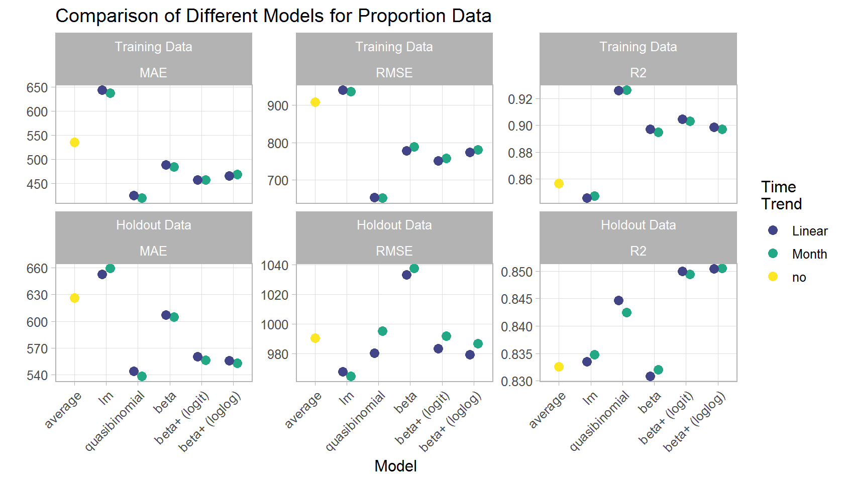
Prediction of Future Matches
Last, I want to make some real predictions, that is, predict the attendance of future matches.
### Model: Beta and Quasibinomial ###

df31 <- filter(df1, date < "2019-05-01") %>%
    mutate(y = transform_perc(perc))

contrasts(df31$home_team) <- contr.sum(levels(df31$home_team))
contrasts(df31$away_team) <- contr.sum(levels(df31$away_team))

res31 <- betareg(y ~ home_team + away_team + weekday + half2*year +
                   Oct + Nov + Dec + Mar + Apr + May | home_team, data = df31)
res32 <- glm(perc ~ home_team + away_team + weekday + half2*year +
                   Oct + Nov + Dec + Mar + Apr + May, data = df31,
             family = quasibinomial(logit), weights = capacity)

# newdata
df32 <- df1 %>%
  filter(season_id == 55149) %>%
  group_by(home_team) %>%
  mutate(avg = round(mean(ifelse(attendance == 0, NA, attendance), na.rm = TRUE), -1)) %>%
  filter(round_number %in% 30:31 & date > as.Date("2019-05-10"))

### Make predictions ###

tab3 <- enframe(list(beta = res31, binomial = res32), "Model") %>%
  mutate(pred = map(value, ~augment(.x, newdata = df32,
                                    type.predict = "resp"))) %>%
  select(-value) %>%
  unnest(pred) %>%
  mutate(prediction = round(.fitted*capacity, -1)) %>%
  select(Model, home_team, away_team, date, capacity, .fitted, prediction, avg) %>%
  pivot_wider(names_from = Model, values_from = .fitted:prediction)

### Prediction interval for beta regression ###

# predict(res31,
#         newdata = filter(df1, season_id == 55149 & round_number == 31),
#         type = "quantile", at = c(.025, .975))

### Make table ###

tab3 %>%
    mutate_at(vars(home_team, away_team),
              ~sub("(-Handewitt)|(Die Eulen )|(FRISCH AUF! )", "", .)) %>%
    mutate_at(vars(home_team, away_team), ~sub("^(\\w{2,4}\\s)+[0-9]*\\s*", "", .)) %>%
    mutate_at(vars(home_team, away_team), ~sub("Burgdorf", "B.", .)) %>%
    mutate_at(vars(home_team, away_team), ~sub("Rhein-Neckar", "R.-N.", .)) %>%
    arrange(date, avg) %>%
    mutate(home_team = sub("(Die Eulen )|(([A-Z]{2,3}\\s)+[0-9]*\\s*)", "", home_team)) %>%
    mutate(away_team = sub("(Die Eulen )|(([A-Z]{2,3}\\s)+[0-9]*\\s*)", "", away_team)) %>%
    select(-.fitted_beta, -.fitted_binomial) %>%
    knitr::kable(digits = 2,
                 col.names = c("Home Team", "Away Team", "Date", "Capacity",
                               "Average", "Beta", "Quasi-B.")) %>%
    kable_styling(bootstrap_options = c("striped", "hover", "condensed", "responsive")) %>%
add_header_above(c(" " = 5, "Predicted Attendance" = 2))| Home Team | Away Team | Date | Capacity | Average | Beta | Quasi-B. |
|---|---|---|---|---|---|---|
| Gummersbach | Lemgo Lippe | 2019-05-11 | 4050 | 3150 | 3770 | 3760 |
| Leipzig | Bergischer HC | 2019-05-11 | 6500 | 4250 | 5100 | 4940 |
| Melsungen | R.-N. Löwen | 2019-05-12 | 4300 | 3910 | 4190 | 4200 |
| Magdeburg | Wetzlar | 2019-05-12 | 7221 | 6410 | 6550 | 6600 |
| Füchse Berlin | Ludwigshafen | 2019-05-12 | 9000 | 7470 | 7900 | 7920 |
| Kiel | Flensburg | 2019-05-12 | 10285 | 10280 | 10280 | 10280 |
| Hannover-B. | Gummersbach | 2019-05-14 | 10000 | 5400 | 8570 | 8140 |
| Ludwigshafen | Stuttgart | 2019-05-15 | 2268 | 2160 | 2160 | 2160 |
| Minden | Leipzig | 2019-05-15 | 4059 | 2730 | 3070 | 3110 |
| Lemgo Lippe | Magdeburg | 2019-05-15 | 4861 | 3640 | 4260 | 4180 |
| Erlangen | Bietigheim | 2019-05-16 | 7850 | 4330 | 4500 | 3630 |
| Flensburg | Melsungen | 2019-05-16 | 6300 | 6030 | 6090 | 6110 |
| R.-N. Löwen | Göppingen | 2019-05-23 | 13200 | 7940 | 8680 | 7980 |
Resources
- Cribari-Neto, F., & Zeileis, A. (2010). Beta regression in R. Journal of Statistical Software, 34(2), 1–24. doi: 10.18637/jss.v034.i02
- Cross Validated: How to do logistic regression in R when outcome is fractional (a ratio of two counts)?
- Cross Validated: What is quasi-binomial distribution (in the context of GLM)?
- There is lot’s of interesting discussion on Cross Validated on whether it makes sense to compute prediction intervals for logistic or binomial regression; see also Prediction intervals for GLMs.