Data with categorical predictors such as groups, conditions, or countries can be analyzed in a regression framework as well as in an ANOVA framework. In either case, the grouping variable needs to be recoded, it cannot enter the model like a continuous predictor such as age or income. A default coding system for categorical variables is often dummy coding.
Even though I usually prefer the more general regression framework, I like the ANOVA perspective because of its focus on meaningful coding schemes beyond dummy coding. Herein, I will illustrate how to use any coding scheme in either framework which will help you (a) to switch between ANOVA and regression and (b) use sensible comparisons of your groups.
In the example below, I use four different groups of people that watched one of four movies, namely, documentary, horror, nature, or comedy.
Regression Perspective
In regression, we often deal with categorical predictors and often a first choice is dummy coding (the default in R for unordered factors). We all know how dummy coding works. Here, we choose “documentary” as a reference category, and all other categories are contrasted with that reference category using the scheme depicted in Table 1. Then, the resulting three estimates give us the difference between “documentary” and each of the three other groups.
| Group | d1 | d2 | d3 |
|---|---|---|---|
| documentary | 0 | 0 | 0 |
| horror | 1 | 0 | 0 |
| nature | 0 | 1 | 0 |
| comedy | 0 | 0 | 1 |
ANOVA and SPSS Perspective
In the ANOVA world or, for example, in experimental psychology, it is often desired to have more tailored comparisons to test specific hypotheses. This can be done using custom contrasts (planned comparisons) as depicted in Table 2. For example, I may investigate the difference between the last group “comedy” and the three other groups using the contrast (-1, -1, -1, 3) depicted in row H1. Furthermore, I may test the difference between “horror” vs. “documentary”+“nature” (H2). Lastly, I may test the difference between “documentary” and “nature”.
| Hypothesis | c1 | c2 | c3 | c4 |
|---|---|---|---|---|
| H1 | -1 | -1 | -1 | 3 |
| H2 | 1 | -2 | 1 | 0 |
| H3 | -1 | 0 | 1 | 0 |
Furthermore, one of the very few things that I like about SPSS is the fact that I can easily define such contrasts using UNIANOVA:
### SPSS Syntax ###
UNIANOVA Y BY X
  /CONTRAST(X) = SPECIAL(-1 -1 -1  3
                          1 -2  1  0
                         -1  0  1  0).
How to Combine the Perspectives?
Even though I was comfortable using either approach, the thing that always bugged me was that I personally wasn’t able to fully bridge the two worlds. For example:
- How can we use such schemes within the other framework?
For example, plugging the dummy codes from Table 1 into SPSS’s
UNIANOVAsyntax won’t work. - How do we actually know the meaning of our estimates? For example, everybody knows that the estimate for the first dummy code “d1” above is the difference between “horror” and “documentary”. But why exactly is this the case?
Solution
The solution is simple, but:
fortunes::fortune("done it.")
#>
#> It was simple, but you know, it's always simple when you've done it.
#>    -- Simone Gabbriellini (after solving a problem with a trick suggested
#>       on the list)
#>       R-help (August 2005)
The solution is that the scheme used in Table 2 above directly defines the contrast matrix C and this allows us to contrast group means in a sensible way. On the other hand, the dummy-coding scheme depicted in Table 1 was a coding matrix B (Venables, 2018). These are two different things and they are related in the following way: \[\beta = \mathbf{C} \mu = \mathbf{B}^{-1} \mu.\] That is, the estimates \(\beta\) are the reparameterized group means \(\mu\). The contrasts in C directly specify the weights of the group means and are easily interpretable. However, the interpretation of the codes in B (e.g., of the dummy codes used above) is not directly given, but only through the inverse of B. This relationship between B and C and the interpretation of the regression coefficients \(\beta\) will be illustrated in the following.
Examples
Example data
I will used a data set called affect from the package psych. Therein, participants watched one of four different films and their positive affect (“PA2”) was assessed afterwards. The plot below shows clearly the effect of films on positive effect. To more formally investigate this effect (using regression or ANOVA), the categorical predictor film has to be recoded into three coding variables; herein, the three schemes dummy, contrast, and Helmert coding will be illustrated. More coding schemes are illustrated on this UCLA page.
# install.packages(c("psych", "ggplot2", "dplyr", "codingMatrices"))
library(ggplot2)
library(dplyr)

data(affect, package = "psych")
# help(affect, package = "psych")

affect$Film <- factor(affect$Film, labels = c("documentary", "horror", "nature", "comedy"))

# Sample subgroups of equal size (n=50)
set.seed(123)
dat <- affect %>%
    group_by(Film) %>%
    sample_n(50)

table(dat$Film)
#>
#> documentary      horror      nature      comedy
#>          50          50          50          50

(group_means <- tapply(dat$PA2, dat$Film, mean))
#> documentary      horror      nature      comedy
#>       8.252       7.060       8.540      12.464

ggplot(dat, aes(y = PA2, x = Film)) +
    stat_summary(fun.data = "mean_cl_normal") +
    labs(y = "Positive Affect ('PA2')") +
    theme_light(base_size = 12) +
    theme(panel.grid.minor = element_blank())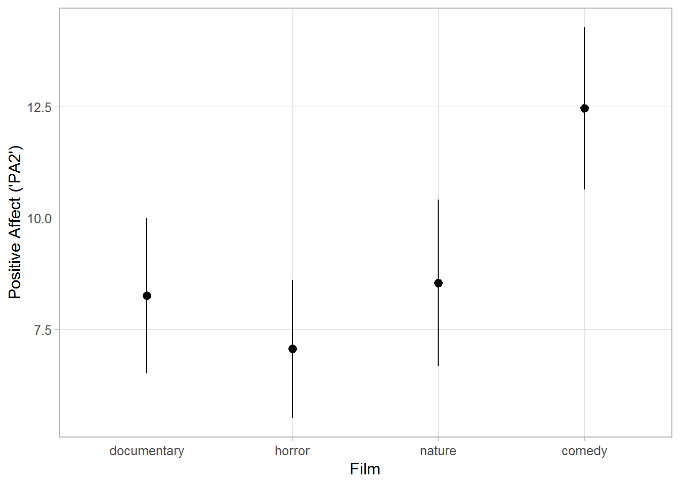
Dummy Coding
Here, we use the default in R, namely, dummy coding, for the affect data. Remember that we want to investigate whether positive affect (“PA2”) differs between groups that watched one of four films. The interpretation of the results is straightforward: The intercept is equal to the mean of the first group “documentary”, and here it is significantly different from zero. Furthermore, we observe that “comedy” in comparison to the reference category “documentary” leads to higher levels of positive effect (the difference is 4.478, p = .0001).
contr.treatment(levels(dat$Film))
#>             horror nature comedy
#> documentary      0      0      0
#> horror           1      0      0
#> nature           0      1      0
#> comedy           0      0      1

summary(lm(PA2 ~ Film, data = dat))
#>
#> Call:
#> lm(formula = PA2 ~ Film, data = dat)
#>
#> Residuals:
#>     Min      1Q  Median      3Q     Max
#> -12.464  -5.060  -1.060   3.748  17.460
#>
#> Coefficients:
#>             Estimate Std. Error t value Pr(>|t|)
#> (Intercept)   8.2520     0.8713   9.471  < 2e-16 ***
#> Filmhorror   -1.1920     1.2322  -0.967 0.334557
#> Filmnature    0.2880     1.2322   0.234 0.815443
#> Filmcomedy    4.2120     1.2322   3.418 0.000767 ***
#> ---
#> Signif. codes:  0 '***' 0.001 '**' 0.01 '*' 0.05 '.' 0.1 ' ' 1
#>
#> Residual standard error: 6.161 on 196 degrees of freedom
#> Multiple R-squared:  0.09987,    Adjusted R-squared:  0.08609
#> F-statistic: 7.249 on 3 and 196 DF,  p-value: 0.000123

group_means
#> documentary      horror      nature      comedy
#>       8.252       7.060       8.540      12.464

12.090 - 7.612       # == 'Filmcomedy'
#> [1] 4.478
But why exactly are the four estimates interpreted in this way?
We learned in stats 101 how to interpret the B matrix depicted in Table 1 (i.e., contr.treatment()).
But to really deduce the meaning, you have to take the inverse of the coding matrix B, which can be done using solve(). (The package codingMatrices has a wrapper around solve() with nice output, but I will use solve() here for transparency.)
# we need to add a vector of 1's for the intercept
solve(cbind(b0 = 1, contr.treatment(4)))
#>     1 2 3 4
#> b0  1 0 0 0
#> 2  -1 1 0 0
#> 3  -1 0 1 0
#> 4  -1 0 0 1

# identical result but nicer ouput:
# codingMatrices::mean_contrasts(contr.treatment(4))
This returns the contrast matrix C. The first row gives you the interpretation of the intercept, and we see that it is \(\beta_0 = 1\mu_1 + 0\mu_2 + 0\mu_3 + 0\mu_4\), namely, the mean of the first group. Likewise, from the second row, \(\beta_1 = -1\mu_1 + 1\mu_2\), that is, the difference between group two and group one; and so on. The interpretation of this C matrix is much easier than that of the B matrix, which was only easy because we learned it by hard.
Lastly, this enables us to use dummy coding (or any other coding scheme that you learned by hard) in SPSS’s UNIANOVA:
### SPSS Syntax ###
UNIANOVA PA2 BY Film
  /CONTRAST(Film) = SPECIAL(-1  1  0  0
                            -1  0  1  0
                            -1  0  0  1).
Planned Comparisons/Contrast Coding
The whole story gets more interesting when trying to implement non-standard coding schemes within the regression framework.
Remember the hypotheses described in Table 2 above; those are easily translated into a contrast matrix C called C1 below.
In order to test the hypotheses within a regression framework, we have to invert C1 to get the B matrix B1.
Furthermore, instead of using integral weights, I divide by the number of non-zero weights for easier interpretation of the estimates (but p-values are the same).
tmp1 <- matrix(c( 1,  1,  1, 1,
                 -1, -1, -1, 3,
                 -1,  2, -1, 0,
                 -1,  0,  1, 0), 4, 4, byrow = TRUE)
C1 <- tmp1 / (4:1)
tmp1
#>      [,1] [,2] [,3] [,4]
#> [1,]    1    1    1    1
#> [2,]   -1   -1   -1    3
#> [3,]   -1    2   -1    0
#> [4,]   -1    0    1    0
round(C1, 2)
#>       [,1]  [,2]  [,3] [,4]
#> [1,]  0.25  0.25  0.25 0.25
#> [2,] -0.33 -0.33 -0.33 1.00
#> [3,] -0.50  1.00 -0.50 0.00
#> [4,] -1.00  0.00  1.00 0.00

B1 <- solve(C1)
round(B1, 2)
#>      [,1]  [,2]  [,3] [,4]
#> [1,]    1 -0.25 -0.33 -0.5
#> [2,]    1 -0.25  0.67  0.0
#> [3,]    1 -0.25 -0.33  0.5
#> [4,]    1  0.75  0.00  0.0

colnames(B1) <- paste0("_Hyp", 0:3)
Finally, we can use the B matrix to test the desired contrasts in a linear regression:
summary(lm(PA2 ~ Film, data = dat, contrasts = list(Film = B1[, -1])))
#>
#> Call:
#> lm(formula = PA2 ~ Film, data = dat, contrasts = list(Film = B1[,
#>     -1]))
#>
#> Residuals:
#>     Min      1Q  Median      3Q     Max
#> -12.464  -5.060  -1.060   3.748  17.460
#>
#> Coefficients:
#>             Estimate Std. Error t value Pr(>|t|)
#> (Intercept)   9.0790     0.4357  20.840  < 2e-16 ***
#> Film_Hyp1     4.5133     1.0061   4.486 1.24e-05 ***
#> Film_Hyp2    -1.3360     1.0671  -1.252    0.212
#> Film_Hyp3     0.2880     1.2322   0.234    0.815
#> ---
#> Signif. codes:  0 '***' 0.001 '**' 0.01 '*' 0.05 '.' 0.1 ' ' 1
#>
#> Residual standard error: 6.161 on 196 degrees of freedom
#> Multiple R-squared:  0.09987,    Adjusted R-squared:  0.08609
#> F-statistic: 7.249 on 3 and 196 DF,  p-value: 0.000123

mean(group_means)
#> [1] 9.079
group_means[[4]] - mean(group_means[1:3])
#> [1] 4.513333
group_means[[2]] - mean(group_means[c(1, 3)])
#> [1] -1.336
group_means[[3]] - group_means[[1]]
#> [1] 0.288
As you can see, the following holds:
- \(\beta_0 = .25\mu_1 +.25\mu_2 +.25\mu_3 + .25\mu_4\),
- \(\beta_1 = -.33\mu_1 -.33\mu_2 -.33\mu_3 + \mu_4\),
- \(\beta_2 = -.5 \mu_1 + \mu_2 -.5\mu_3\),
- \(\beta_3 = - \mu_1 + \mu_3\).
Thus, positive affect is 4.41 points higher after watching “comedy” compared to the three other films (p < .001). Moreover, positive affect is 0.33 points lower after “horror” compared to groups 1 and 3, but this is not significant (p = .742). And the difference between “documentary”" and “nature” is also non-significant (p = .760).
This gives us huge power.
We can now test more specific hypotheses in a regression framework compared to what is possible using the software’s defaults.
For example, the hypotheses depicted in Table 2 were easy to test using our custom matrices B1 and C1 but would be hard to test with built-in functions.
Furthermore, we know now how to deduce the meaning of the estimates instead of relying on textbook knowledge.
Helmert Coding
For further illustration, we will have a look at Helmert coding (contr.helmert()), which can be used to compare each level with the mean of the previous levels.
The C matrix C2 below already illustrates that, but it does not give an interpretation for \(\beta_0\) and it does not allow to interpret the exact value of the other estimates.
This is given by its inverse B2, which shows that \(\beta_0\) is again the mean of the group means (first row of B2). Furthermore, \(\beta_3\) compares “comedy” to the three other groups (H1 in Table 2), and the p- and t-value (4.742) are the same as above.
However, the estimate of 1.10 has no easy interpretation, because it is \(\beta_3 = -0.08\mu_1 - 0.08\mu_2 - 0.08\mu_3 + 0.25\mu_4\).
This was much easier to interpret above, where the estimate was 4.41, which was just the difference between “comedy” and the mean of the other three groups.
(C2 <- contr.helmert(levels(dat$Film)))
#>             [,1] [,2] [,3]
#> documentary   -1   -1   -1
#> horror         1   -1   -1
#> nature         0    2   -1
#> comedy         0    0    3

B2 <- solve(cbind(1, C2))
round(B2, 2)
#>      documentary horror nature comedy
#> [1,]        0.25   0.25   0.25   0.25
#> [2,]       -0.50   0.50   0.00   0.00
#> [3,]       -0.17  -0.17   0.33   0.00
#> [4,]       -0.08  -0.08  -0.08   0.25

summary(lm(PA2 ~ Film, data = dat, contrasts = list(Film = contr.helmert)))
#>
#> Call:
#> lm(formula = PA2 ~ Film, data = dat, contrasts = list(Film = contr.helmert))
#>
#> Residuals:
#>     Min      1Q  Median      3Q     Max
#> -12.464  -5.060  -1.060   3.748  17.460
#>
#> Coefficients:
#>             Estimate Std. Error t value Pr(>|t|)
#> (Intercept)   9.0790     0.4357  20.840  < 2e-16 ***
#> Film1        -0.5960     0.6161  -0.967    0.335
#> Film2         0.2947     0.3557   0.828    0.408
#> Film3         1.1283     0.2515   4.486 1.24e-05 ***
#> ---
#> Signif. codes:  0 '***' 0.001 '**' 0.01 '*' 0.05 '.' 0.1 ' ' 1
#>
#> Residual standard error: 6.161 on 196 degrees of freedom
#> Multiple R-squared:  0.09987,    Adjusted R-squared:  0.08609
#> F-statistic: 7.249 on 3 and 196 DF,  p-value: 0.000123

sum(B2[4, ] * group_means)
#> [1] 1.128333
Orthogonal and Nonorthognoal Contrasts
I did not find much literature that deduces the meaning of the B matrix and explains the relationship between B and C except Venables (2018). Maybe because it is obvious for everyone except for me. But maybe because people are taught to use either standard schemes (like dummy coding) or orthogonal contrasts. Orthogonal contrasts have the advantage that they can be interpreted using either the B or the C matrix, because they are structurally quite similar, and thus no one needs to know about or calculate an inverse:
# B matrix for Helmert coding
contr.helmert(5)
#>   [,1] [,2] [,3] [,4]
#> 1   -1   -1   -1   -1
#> 2    1   -1   -1   -1
#> 3    0    2   -1   -1
#> 4    0    0    3   -1
#> 5    0    0    0    4

# C matrix
tmp1 <- solve(cbind(1, contr.helmert(5)))[-1, ]
round(t(tmp1), 2)
#>   [,1]  [,2]  [,3]  [,4]
#> 1 -0.5 -0.17 -0.08 -0.05
#> 2  0.5 -0.17 -0.08 -0.05
#> 3  0.0  0.33 -0.08 -0.05
#> 4  0.0  0.00  0.25 -0.05
#> 5  0.0  0.00  0.00  0.20
I don’t know of any other clear advantages of orthogonal over nonorthogonal contrasts. If you know better, I would be very happy if you could let me know.
References
Venables, B. (2018). Coding matrices, contrast matrices and linear models. Retrieved from https://cran.r-project.org/web/packages/codingMatrices/vignettes/