Lowest Number of Red Cards in 40 Years

Scraping Data for One Year

I will use the rvest package here, which makes it pretty easy to get the data from http://www.thesoccerworldcups.com. There are more comprehensive tutorials on the web, so I will just focus on this single example. As you can see below, the webpage is first given to read_html(). Second, one has to identify which part of the page is relevant using CSS selectors. SelectorGadget is a recommended tool to do this, or you may directly inspect the page source. Here, the node name is “.c0s5”, and this information is passed to html_nodes(). Third, the information of interest can be extracted using another html_*() function. Luckily, thesoccerworldcups.com uses tables to store the data so that we can use html_table(), which leads to results that need little wrangling. Alternatively, html_text() can be used which returns a character vector.

tmp1 <- read_html("http://www.thesoccerworldcups.com/world_cups/2018_cards.php")
    
tmp2 <- html_nodes(tmp1, ".c0s5")
tmp3 <- html_table(tmp2, header = TRUE, fill = TRUE)

tmp4 <- tmp3[[1]]

tmp4[28:32, 3:7]
#>                 Player Yellow Cards Red Cards (SRC / 2YC) Games
#> 28      Blaise Matuidi            2         -           -     5
#> 29       Kylian Mbappé            2         -           -     7
#> 30              Player Yellow Cards Red Cards (SRC / 2YC) Games
#> 31      Thomas Meunier            2         -           -     5
#> 32 Aleksandar Mitrovic            2         -           -     3

str(tmp4, 2)
#> 'data.frame':    192 obs. of  10 variables:
#>  $              : chr  "" "" "" "" ...
#>  $              : chr  "Carlos Sánchez" "Jérôme Boateng" "Michael Lang" "Igor Smolnikov" ...
#>  $ Player       : chr  "Carlos Sánchez" "Jérôme Boateng" "Michael Lang" "Igor Smolnikov" ...
#>  $ Yellow Cards : chr  "1" "-" "-" "-" ...
#>  $ Red Cards    : chr  "1" "1" "1" "1" ...
#>  $ (SRC / 2YC)  : chr  "( 1   \r\n\t\t\t/\r\n\t\t\t -\t\t\t)" "( -   \r\n\t\t\t/\r\n\t\t\t 1\t\t\t)" "( 1   \r\n\t\t\t/\r\n\t\t\t -\t\t\t)" "( -   \r\n\t\t\t/\r\n\t\t\t 1\t\t\t)" ...
#>  $ Games        : chr  "3" "2" "3" "1" ...
#>  $ National Team: chr  "Colombia" "Germany" "Switzerland" "Russia" ...
#>  $ NA           : logi  NA NA NA NA NA NA ...
#>  $ NA           : logi  NA NA NA NA NA NA ...

As you see, we actually managed to retrieve the relevant information using only three function calls. Furthermore, the data is stored in a data frame that looks very similar to the one on thesoccerworldcups.com. We have a tidy data frame with a column for every variable and a row for every player. Nevertheless, a few things need to be done:

• Some columns have no or bad names. Address using make.names().
• The column names are repeated in every 30th row. Address using filter().
• Some columns should be integers instead of characters. Address using as.integer().
• There is a single column “(SRC / 2YC)” that stores two information, namely, whether a red card was either a straight red card (SRC) or the result of two yellow cards (2YC). This needs to be split into two variables using separate(). But first, all the unnecessary characters like \n\t\t\t in that column must be removed using gsub() with a regular expression.
• Several columns contain no relevant information and can be dropped.
• The last two rows contain the information for the whole World Cup not for individual players.

names(tmp4) <- make.names(names(tmp4), unique = TRUE)

tmp5 <- dplyr::filter(tmp4, Player != "Player")

tmp5$Yellow.Cards <- as.integer(tmp5$Yellow.Cards)
tmp5$Red.Cards    <- as.integer(tmp5$Red.Cards)
tmp5$Games        <- as.integer(tmp5$Games)

tmp5$X.SRC...2YC. <- gsub("\\s*|[(]|[)]", "", tmp5$X.SRC...2YC.)
tmp6 <- tidyr::separate(tmp5, X.SRC...2YC., c("SRC", "2YC"),
                        convert = TRUE, fill = "right")

psych::headTail(tmp6[, 3:9])
#>             Player Yellow.Cards Red.Cards  SRC X2YC Games National.Team
#> 1   Carlos Sánchez            1         1    1 <NA>     3      Colombia
#> 2   Jérôme Boateng         <NA>         1 <NA>    1     2       Germany
#> 3     Michael Lang         <NA>         1    1 <NA>     3   Switzerland
#> 4   Igor Smolnikov         <NA>         1 <NA>    1     1        Russia
#> ...           <NA>          ...       ...  ...  ...   ...          <NA>
#> 183  Denis Zakaria            1      <NA> <NA> <NA>     2   Switzerland
#> 184   Roman Zobnin            1      <NA> <NA> <NA>     5        Russia
#> 185                        <NA>      <NA> <NA> <NA>  <NA>              
#> 186        Totals:          219         4    2    2  <NA>
    
dat1 <- tmp6[1:(nrow(tmp6)-2), ]

dat2 <- tmp6[nrow(tmp6), ]

Now, all information about yellow and red cards are available for one year. This can be repeated for the other tournaments.

I also scrape the data of the final standings from http://www.thesoccerworldcups.com/world_cups/2018_final_standings.php. This gives me the information about how many matches a team played allowing me to calculate the number of cards per match for each team individually. These two data frames can then be merged/joined

Scraping Data for All Years

In the code below, the data for all tournaments since 1966 are scraped in a loop. Furthermore, a little data wrangling is done, but I won’t bother you with the details here.

years <- seq(1966, 2018, by = 4)

list1 <- vector("list", length = length(years))
names(list1) <- years

for (ii in seq_along(years)) {
    tmp1 <- read_html(sprintf(
        "http://www.thesoccerworldcups.com/world_cups/%d_cards.php",
        years[ii]))
    
    tmp2 <- html_nodes(tmp1, ".c0s5")
    tmp3 <- html_table(tmp2, header = TRUE, fill = TRUE)
    
    tmp4 <- tmp3[[1]]
    names(tmp4) <- make.names(names(tmp4), unique = TRUE)
    tmp5 <- tmp4 %>% 
        dplyr::filter(Player != "Player") %>% 
        {suppressWarnings(dplyr::mutate_at(., dplyr::vars(Yellow.Cards, Red.Cards, Games),
                                           as.integer))} %>%
        dplyr::select(Player:National.Team)
    
    tmp5$X.SRC...2YC. <- gsub("\\s*|[(]|[)]", "", tmp5$X.SRC...2YC.)
    tmp6 <- tidyr::separate(tmp5, X.SRC...2YC., c("SRC", "2YC"),
                            convert = TRUE, fill = "right")
    
    dat1 <- tmp6[1:(nrow(tmp6) - 2), ]
    dat2 <- tmp6[nrow(tmp6), ]
    
    if (any(c(sum(dat1$Yellow.Cards, na.rm = TRUE) != dat2$Yellow.Cards,
              sum(dat1$Red.Cards, na.rm = TRUE) != dat2$Red.Cards,
              sum(dat1$SRC, na.rm = TRUE) != dat2$SRC,
              sum(dat1$`2YC`, na.rm = TRUE) != dat2$`2YC`))) {
        stop("Sums do not match")
    }
    
    ttmp1 <- read_html(sprintf(
        "http://www.thesoccerworldcups.com/world_cups/%d_final_standings.php",
        years[ii]))
    
    ttmp2 <- html_nodes(ttmp1, ".c0s5")
    ttmp3 <- html_table(ttmp2, header = TRUE, fill = TRUE)[[1]]
    
    ttmp4 <- ttmp3[complete.cases(ttmp3[, 1:(ncol(ttmp3) - 2)]),
                   1:(ncol(ttmp3) - 2)]
    names(ttmp4) <- make.names(names(ttmp4), unique = TRUE)
    
    dat1$WC_games <- sum(ttmp4$GP, na.rm = TRUE)/2
    
    dat3 <- ttmp4 %>% 
        dplyr::select(-Standing) %>% 
        dplyr::right_join(dat1, by = "National.Team")
    
    list1[[ii]] <- dat3
}

gdata::keep(years, list1, sure = TRUE)

data1 <- reshape2::melt(list1,
                        measure.vars = c("Yellow.Cards", "Red.Cards",
                                         "SRC", "2YC"))
names(data1) <- sub("L1", "Year", names(data1))
data1$Year <- as.integer(data1$Year)

data1$National.Team <- forcats::fct_collapse(data1$National.Team,
                                             Germany = "West Germany")
data1$variable <- factor(data1$variable,
                         levels = c("Yellow.Cards", "Red.Cards", "2YC", "SRC"),
                         labels = c("Yellow Cards", "Red Cards", "2YC", "SRC"))

Calculating the Number of Cards

In its current form, the data stores information about cards for individual players. However, I am interested in the number of cars per tournament, and in the number of cards per team. Moreover, I want to investigate not total cards but cards per match. The relevant information is calculated below. Note that “cards per team” is not twice the number of “cards per match”, since some teams played more games than others.

data_wc <- data1 %>% 
    dplyr::group_by(Year, variable, WC_games) %>%
    dplyr::summarize(Cards = sum(value, na.rm = TRUE)) %>% 
    dplyr::mutate(CardsPerMatch = Cards/WC_games) %>% 
    dplyr::arrange(dplyr::desc(Year))

data_teams <- data1 %>% 
    dplyr::group_by(Year, National.Team, variable, GP) %>% 
    dplyr::summarize(cards = sum(value, na.rm = TRUE)) %>%
    dplyr::mutate(CardsPerMatch = cards/GP) %>% 
    dplyr::arrange(dplyr::desc(Year))

Results

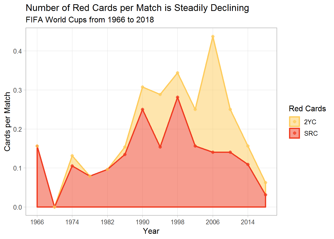
The results confirmed my impression. There were only four red cards in 2018, which is an average of 0.06 per match. This is the lowest number since 1974, and we see a steady decrease since a peek in 2006. This holds for both straight red cards (SRC) and two yellow cards (2YC).

data_wc %>% 
    dplyr::filter(variable %in% c("SRC", "2YC")) %>% 
    ggplot(aes(x = Year, y = CardsPerMatch, fill = variable, col = variable)) +
    geom_area(alpha = .5, size = 1) +
    geom_point(position = "stack", alpha = .75, size = 2) +
    scale_fill_manual(values = c("#fecc5c", "#f03b20")) +
    scale_color_manual(values = c("#fecc5c", "#f03b20")) +
    scale_x_continuous(breaks = seq(1966, 2018, by = 8)) +
    labs(fill = "Red Cards", col = "Red Cards", x = "Year",
         y = "Cards per Match",
         title = "Number of Red Cards per Match is Steadily Declining",
         subtitle = "FIFA World Cups from 1966 to 2018"
         # , caption = "Data from http://www.thesoccerworldcups.com/"
         )

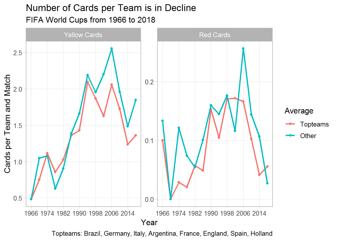
And this holds also within teams: Similar patterns are observed for the eight most successful teams compared to all other teams as shown below.

For yellow cards, the pattern is less clear. There were fewer yellow cards compared to 1994–2010, but more than in 2014.

While my gut feeling about the decline of red cards was right, I have no final explanation. Players are maybe less emotional and more focused these days. But habits of referees or rules and other things may have changed as well.

topteams <- c("Brazil", "Germany", "Italy", "Argentina",
              "France", "England", "Spain", "Holland")

data_teams$Team <- forcats::fct_other(data_teams$National.Team, keep = topteams)
data_teams$Team <- forcats::fct_other(data_teams$Team, keep = "Other", other_level = "Topteams")
data_teams$Team <- forcats::fct_rev(data_teams$Team)

datax <- data_teams %>% 
    dplyr::group_by(Year, Team, variable) %>%
    dplyr::filter(variable %in% c("Yellow Cards", "Red Cards")) %>% 
    dplyr::summarise(CardsPerTeam = mean(CardsPerMatch))

ggplot(datax, aes(x = Year, y = CardsPerTeam, col = Team)) +
    facet_wrap( ~ variable, scales = "free_y") +
    geom_point() +
    geom_line(size = 1) +
    scale_x_continuous(breaks = seq(1966, 2018, by = 8)) +
    labs(y = "Cards per Team and Match",
         col = "Average",
         title = "Number of Cards per Team is in Decline",
         subtitle = "FIFA World Cups from 1966 to 2018",
         caption = paste("Topteams:", paste(topteams, collapse = ", ")))