Recently, I wrote a summary of some illustrative IRT analyses for my students. Quickly, I realized that this might be of interest to others as well, and I am posting here a tutorial for the Rasch model and the 2PL model in R. It is meant for people with a basic understanding of these models who have heard terms like ICC or item difficulty before and who would like to see a practical, worked example. Possibly, the code may be copied and applied to your own data. Let me know if there is anything that needs further clarification.
Setup
Herein, we will use the following three R packages: eRm (Mair & Hatzinger, 2007), ltm (Rizopoulos, 2006), and difR (Magis, Béland, Tuerlinckx, & De Boeck, 2010). Those need to be loaded via library() and installed beforehand if necessary.
# install.packages("eRm")
# install.packages("ltm")
# install.packages("difR")
library("eRm")
library("ltm")
library("difR")
Data
An illustrative data set on verbal aggression will be used, which is comprised of 24 dichotomized items and 316 persons. The data set called verbal is included in the difR package and can be loaded using the function data(). Documentation for the data is available through ?verbal.
data(verbal, package = "difR")
# ?verbal
Rasch Model
A Rasch model is fit to the data using conditional maximum likelihood (CML) estimation of the item parameters as provided in the function RM() of the eRm package.
The item difficulty parameters are returned and the output shows that S2WantCurse is the easiest item and S3DoShout is the most difficult item, for which only people with high levels of verbal aggression are expected to agree with.
dat_1 <- verbal[, 1:24]

res_rm_1 <- RM(dat_1)

# res_rm_1                   # Short summary of item parameters
# summary(res_rm_1)          # Longer summary of item parameters
betas <- -coef(res_rm_1)     # Item difficulty parameters
round(sort(betas), 2)
#> beta S2WantCurse   beta S1DoCurse beta S1wantCurse beta S4WantCurse
#>            -1.91            -1.38            -1.38            -1.25
#>   beta S2DoCurse   beta S4DoCurse beta S2WantScold beta S1WantScold
#>            -1.04            -0.87            -0.87            -0.73
#> beta S3WantCurse   beta S1DoScold beta S1WantShout beta S2WantShout
#>            -0.70            -0.56            -0.25            -0.18
#>   beta S2DoScold   beta S3DoCurse beta S4WantScold   beta S4DoScold
#>            -0.11             0.04             0.18             0.21
#> beta S3WantScold   beta S1DoShout beta S4WantShout   beta S2DoShout
#>             0.51             0.70             0.87             1.31
#>   beta S3DoScold beta S3WantShout   beta S4DoShout   beta S3DoShout
#>             1.33             1.36             1.84             2.87
Plots
We may plot the ICC of a single or all items, which is just a graphical illustration of the estimated item parameters.
plotICC(res_rm_1, item.subset = "S2WantShout")
abline(v = -0.18, col = "grey")
abline(h = .5, col = "grey")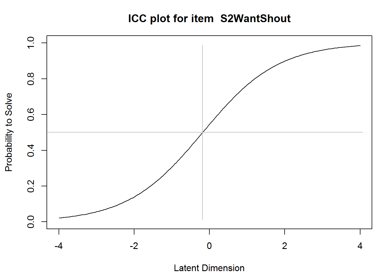
plotjointICC(res_rm_1, item.subset = 1:12, cex = .6)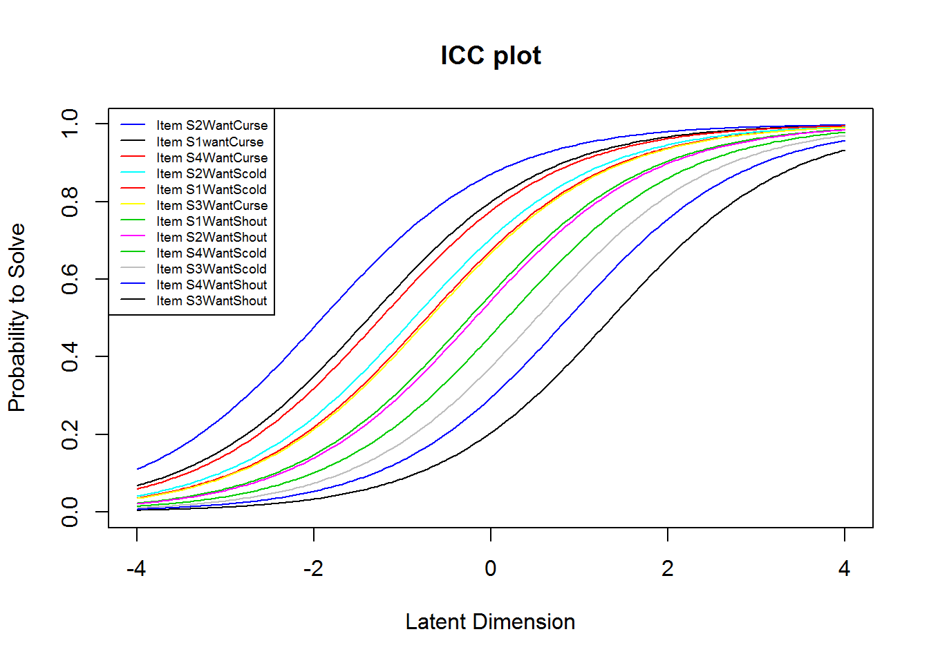
plotjointICC(res_rm_1, item.subset = 13:24, cex = .6)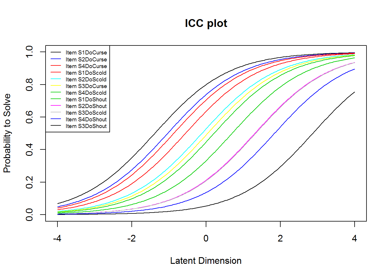
From the plots of the ICCs, it seems like the “want”-items (items 1:12) are easier than the “do”-items (items 13:24). We may further investigate this by comparing the means of the item difficulties. This shows that this is indeed the case. (The two means sum to 0, because of the identification constraint, see below.)
mean(betas[ 1:12])           # Want-items
#> [1] -0.3622058
mean(betas[13:24])           # Do-items
#> [1] 0.3622058
Furthermore, a very informative plot called a person-item map is available in eRm:
A person-item map displays the location of item (and threshold) parameters as well as the distribution of person parameters.along the latent dimension. Person-item maps are useful to compare the range and position of the item measure distribution (lower panel) to the range and position of the person measure distribution (upper panel). Items should ideally be located along the whole scale to meaningfully measure the ‘ability’ of all persons. (From
?plotPImap)
plotPImap(res_rm_1, cex.gen = .55)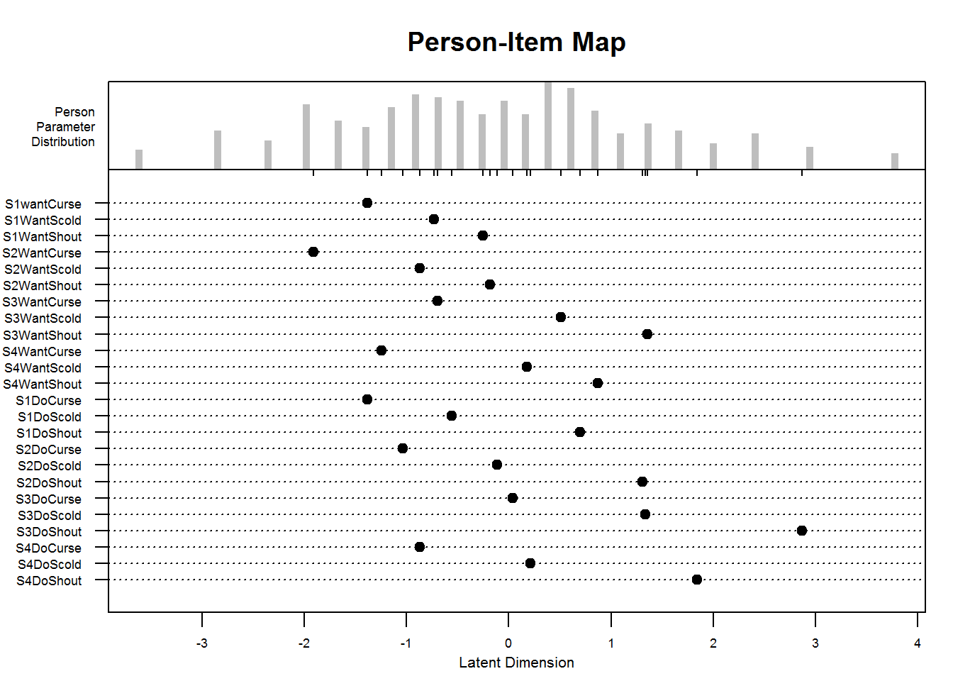
plotPImap(res_rm_1, cex.gen = .55, sorted = TRUE)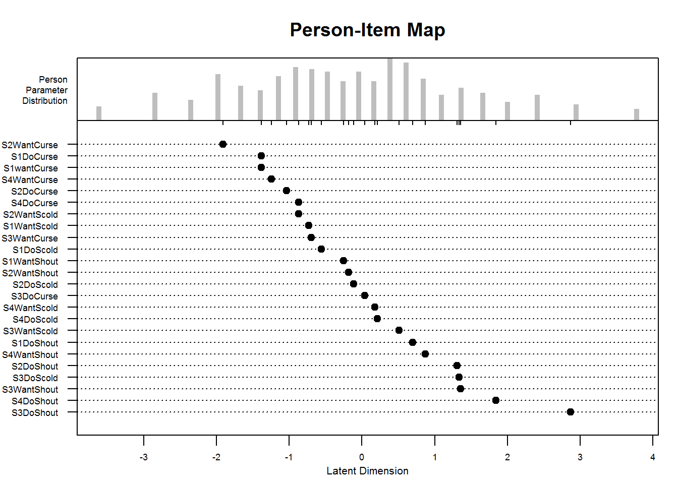
Model Identification
The model needs an identification constraint, because otherwise the location of the latent scale is undetermined. When looking at the help (?RM), we can see that the identification constraint in RM() is a sum-to-zero constraint by default (sum0 = TRUE). We can verify that by calculating the sum of the item parameters.
round(sum(betas), 10)
#> [1] 0
When setting sum0 = FALSE, the first item parameter is set to zero. These are the only two options implemented in RM().
tmp1 <- RM(dat_1, sum0 = FALSE)
round(coef(tmp1), 2)
#> beta S1wantCurse beta S1WantScold beta S1WantShout beta S2WantCurse
#>             0.00            -0.65            -1.13             0.53
#> beta S2WantScold beta S2WantShout beta S3WantCurse beta S3WantScold
#>            -0.51            -1.20            -0.69            -1.90
#> beta S3WantShout beta S4WantCurse beta S4WantScold beta S4WantShout
#>            -2.74            -0.14            -1.56            -2.25
#>   beta S1DoCurse   beta S1DoScold   beta S1DoShout   beta S2DoCurse
#>             0.00            -0.83            -2.08            -0.35
#>   beta S2DoScold   beta S2DoShout   beta S3DoCurse   beta S3DoScold
#>            -1.27            -2.70            -1.42            -2.72
#>   beta S3DoShout   beta S4DoCurse   beta S4DoScold   beta S4DoShout
#>            -4.25            -0.51            -1.60            -3.22
Note on Item Parameters in eRm Package
Note that the eRm package works with easiness parameters, which are called beta, and those can be transformed into difficulty parameters, which are called eta, and \(-\eta = \beta\).
Note further that often only \(I-1\) item parameters are returned (here 23), which illustrates the fact that only 23 item parameters can be estimated and that one has to be fixed either as \(\beta_1=\sum_2^I \beta_i\) (if sum0 = TRUE) or \(\beta_1 = 0\) (if sum0 = FALSE). The first item parameter can then be calculated (not estimated) accordingly.
# No difficulty (eta) parameter is returned for the first item S1wantCurse
summary(res_rm_1)
#>
#> Results of RM estimation:
#>
#> Call:  RM(X = dat_1)
#>
#> Conditional log-likelihood: -3049.923
#> Number of iterations: 31
#> Number of parameters: 23
#>
#> Item (Category) Difficulty Parameters (eta): with 0.95 CI:
#>             Estimate Std. Error lower CI upper CI
#> S1WantScold   -0.731      0.131   -0.987   -0.475
#> S1WantShout   -0.249      0.128   -0.501    0.003
#> S2WantCurse   -1.909      0.153   -2.210   -1.608
#> S2WantScold   -0.873      0.132   -1.132   -0.614
#> S2WantShout   -0.181      0.128   -0.433    0.070
#> S3WantCurse   -0.696      0.130   -0.951   -0.440
#> S3WantScold    0.514      0.132    0.254    0.773
#> S3WantShout    1.358      0.149    1.065    1.650
#> S4WantCurse   -1.245      0.137   -1.514   -0.976
#> S4WantScold    0.178      0.129   -0.076    0.432
#> S4WantShout    0.871      0.138    0.601    1.141
#> S1DoCurse     -1.383      0.140   -1.658   -1.109
#> S1DoScold     -0.557      0.129   -0.810   -0.303
#> S1DoShout      0.698      0.135    0.434    0.963
#> S2DoCurse     -1.037      0.134   -1.300   -0.774
#> S2DoScold     -0.113      0.128   -0.365    0.138
#> S2DoShout      1.312      0.148    1.022    1.602
#> S3DoCurse      0.040      0.129   -0.212    0.293
#> S3DoScold      1.335      0.149    1.044    1.626
#> S3DoShout      2.871      0.222    2.436    3.306
#> S4DoCurse     -0.873      0.132   -1.132   -0.614
#> S4DoScold      0.213      0.130   -0.042    0.467
#> S4DoShout      1.840      0.165    1.516    2.165
#>
#> Item Easiness Parameters (beta) with 0.95 CI:
#>                  Estimate Std. Error lower CI upper CI
#> beta S1wantCurse    1.383      0.140    1.109    1.658
#> beta S1WantScold    0.731      0.131    0.475    0.987
#> beta S1WantShout    0.249      0.128   -0.003    0.501
#> beta S2WantCurse    1.909      0.153    1.608    2.210
#> beta S2WantScold    0.873      0.132    0.614    1.132
#> beta S2WantShout    0.181      0.128   -0.070    0.433
#> beta S3WantCurse    0.696      0.130    0.440    0.951
#> beta S3WantScold   -0.514      0.132   -0.773   -0.254
#> beta S3WantShout   -1.358      0.149   -1.650   -1.065
#> beta S4WantCurse    1.245      0.137    0.976    1.514
#> beta S4WantScold   -0.178      0.129   -0.432    0.076
#> beta S4WantShout   -0.871      0.138   -1.141   -0.601
#> beta S1DoCurse      1.383      0.140    1.109    1.658
#> beta S1DoScold      0.557      0.129    0.303    0.810
#> beta S1DoShout     -0.698      0.135   -0.963   -0.434
#> beta S2DoCurse      1.037      0.134    0.774    1.300
#> beta S2DoScold      0.113      0.128   -0.138    0.365
#> beta S2DoShout     -1.312      0.148   -1.602   -1.022
#> beta S3DoCurse     -0.040      0.129   -0.293    0.212
#> beta S3DoScold     -1.335      0.149   -1.626   -1.044
#> beta S3DoShout     -2.871      0.222   -3.306   -2.436
#> beta S4DoCurse      0.873      0.132    0.614    1.132
#> beta S4DoScold     -0.213      0.130   -0.467    0.042
#> beta S4DoShout     -1.840      0.165   -2.165   -1.516

# Calculate eta for item S1wantCurse
-sum(res_rm_1$etapar)
#> [1] -1.383377
MML Estimation
In contrast to the CML estimation above, the model is now fit using marginal maximum likelihood (MML) estimation using the function rasch() from the ltm package. Therein, the model is identified by assuming a standard normal distribution of the person parameters. Thus, all item parameters can be freely estimated because the mean of the person parameters is fixed to 0 (which was not the case with CML).
res_rm_2 <- rasch(dat_1)
res_rm_2
#>
#> Call:
#> rasch(data = dat_1)
#>
#> Coefficients:
#> Dffclt.S1wantCurse  Dffclt.S1WantScold  Dffclt.S1WantShout
#>             -0.889              -0.409              -0.055
#> Dffclt.S2WantCurse  Dffclt.S2WantScold  Dffclt.S2WantShout
#>             -1.274              -0.513              -0.005
#> Dffclt.S3WantCurse  Dffclt.S3WantScold  Dffclt.S3WantShout
#>             -0.383               0.505               1.120
#> Dffclt.S4WantCurse  Dffclt.S4WantScold  Dffclt.S4WantShout
#>             -0.787               0.259               0.767
#>   Dffclt.S1DoCurse    Dffclt.S1DoScold    Dffclt.S1DoShout
#>             -0.888              -0.281               0.641
#>   Dffclt.S2DoCurse    Dffclt.S2DoScold    Dffclt.S2DoShout
#>             -0.634               0.045               1.087
#>   Dffclt.S3DoCurse    Dffclt.S3DoScold    Dffclt.S3DoShout
#>              0.158               1.103               2.176
#>   Dffclt.S4DoCurse    Dffclt.S4DoScold    Dffclt.S4DoShout
#>             -0.513               0.285               1.464
#>             Dscrmn
#>              1.368
#>
#> Log.Lik: -4037.402
Note further that rasch() did not only fix the mean of the person-parameter distribution, but also the variance. Thus, the variability or units of the latent scale are determined by this. With CML estimation, this was fixed by assuming discrimination parameters equal to 1. However, two constraints (variance of person-parameter distribution as well as discrimination parameter) would be overly restrictive, and thus a common discrimination parameter is freely estimated by rasch(), which equals 1.37. Don’t get distracted by these technical issues, the software takes care of it.
The difficulty parameters estimated via MML or CML are nearly identical here highlighting the fact that the normal-distribution assumption in MML did not do any harm.
cor(coef(res_rm_2)[, 1], betas)
#> [1] 0.9999381
2PL Model
A 2PL model cannot be estimated with eRm, but with the package ltm, for example.
The estimated difficulty parameters (Dffclt) seem roughly comparable to those from the Rasch model. The discrimination parameters (Dscrmn), which were all equal in the Rasch model, show some but not massive heterogeneity. This is also evident from the plot of the ICCs.
Note that res_2pl_1 and res_rm_1 were estimated using two different packages. Thus, the structure of these objects is completely different and also the output if they are printed or the functions you may use with them (e.g., plot() vs. plotICC()).
# ltm() takes a formula with a tilde (~) as its first argument. The left-hand side
# must be the data and the right-hand side are the latent variables (only one
# here).
res_2pl_1 <- ltm(dat_1 ~ z1)
res_2pl_1
#>
#> Call:
#> ltm(formula = dat_1 ~ z1)
#>
#> Coefficients:
#>              Dffclt  Dscrmn
#> S1wantCurse  -0.913   1.358
#> S1WantScold  -0.409   1.525
#> S1WantShout  -0.078   1.340
#> S2WantCurse  -1.243   1.468
#> S2WantScold  -0.500   1.567
#> S2WantShout  -0.026   1.249
#> S3WantCurse  -0.531   0.880
#> S3WantScold   0.475   1.409
#> S3WantShout   1.455   0.912
#> S4WantCurse  -0.906   1.129
#> S4WantScold   0.214   1.588
#> S4WantShout   0.946   0.967
#> S1DoCurse    -0.821   1.666
#> S1DoScold    -0.251   2.272
#> S1DoShout     0.605   1.420
#> S2DoCurse    -0.630   1.475
#> S2DoScold     0.009   1.987
#> S2DoShout     0.968   1.625
#> S3DoCurse     0.164   1.089
#> S3DoScold     1.098   1.342
#> S3DoShout     2.457   1.126
#> S4DoCurse    -0.537   1.363
#> S4DoScold     0.255   1.430
#> S4DoShout     1.592   1.180
#>
#> Log.Lik: -4017.413

# ?plot.ltm
plot(res_2pl_1, items =  1:12)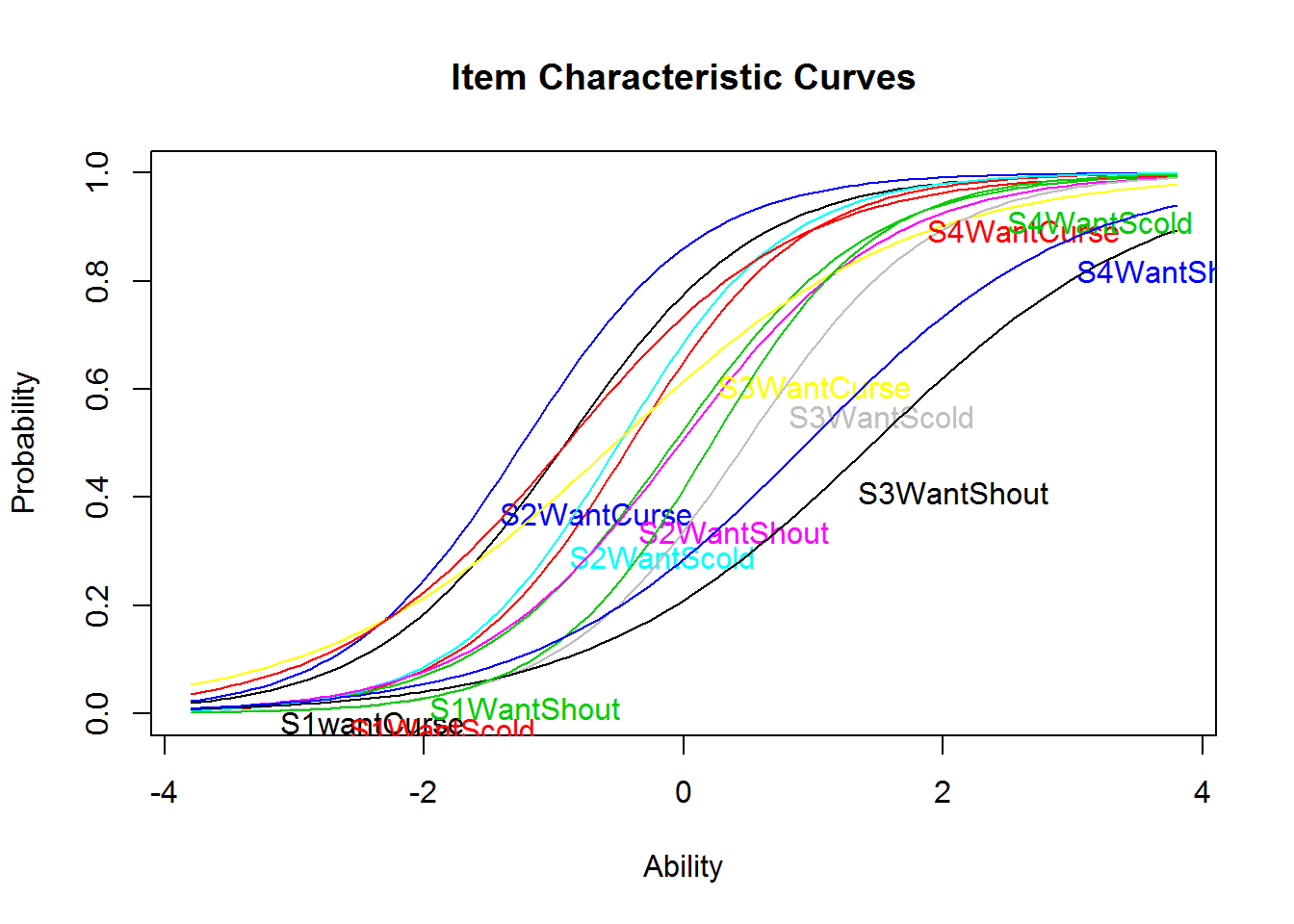
plot(res_2pl_1, items = 13:24)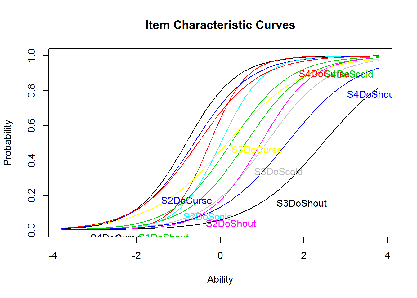
Model Fit
Relative Fit of Rasch and 2PL Model
To compare the Rasch and the 2PL model, both need to be fit using the same assumptions and the same algorithm. Therefore, the comparison is made here based on the models estimated via MML.
Likelihood-Ratio Test
Since the two models are nested, they can be compared using a Likelihood-Ratio (LR) test. Here, the test is significant (p = .015) indicating that both models do not fit equally well and that the more complex 2PL model is preferred.
Note that a model with more parameters always leads to a higher likelihood, which is also the case here. Note further, that the degrees of freedom (df) for the LR test equal the number of constrained parameters. In the 2PL model, 24 discrimination parameters were estimated, and in the Rasch model only 1, which gives df = 23.
anova(res_rm_2, res_2pl_1)
#>
#>  Likelihood Ratio Table
#>               AIC    BIC  log.Lik   LRT df p.value
#> res_rm_2  8124.80 8218.7 -4037.40
#> res_2pl_1 8130.83 8311.1 -4017.41 39.98 23   0.015
AIC and BIC
To compare two models descriptively, they need not necessarily be nested. With respect to AIC and BIC, lower values indicate better fit. Herein, the Rasch model is preferred by both criteria.
Comparison of Item Parameters
To further evaluate differences between the two models, the difficulty parameters can be correlated across models. Again, the extremely high correlation indicates that the differences between models is small.
cor(coef(res_rm_2)[, 1], coef(res_2pl_1)[, 1])
#> [1] 0.9942499
Absolute Fit of the Rasch Model
In the remainder of this subsection, a few procedures for assessing the fit of the Rasch model will be illustrated.
Several of them are based on the idea that the item parameters—estimated separately in two groups—should be equal if the model holds. For illustrative purposes, the variable sex is used here but other/additional variables can of course be used.
Andersen’s Likelihood-Ratio Test and Graphical Model Check
The item parameters should be equal if the model holds and thus be close to the line in the following plot. The ellipses indicate the confidence intervals, and many of them overlap the line indicating good fit. A few items stand out, for example item 6 (S2WantShout), which is easier for women than for men.
The significance test that formalizes this idea is called Andersen’s Likelihood Ratio test (Andersen, 1973). Herein, it is significant indicating bad fit due to too many items with diverging item difficulties.
lrt_1 <- LRtest(res_rm_1, splitcr = verbal$Gender)
plotGOF(lrt_1, conf = list(), tlab = "number",
        xlab = "Women", ylab = "Men")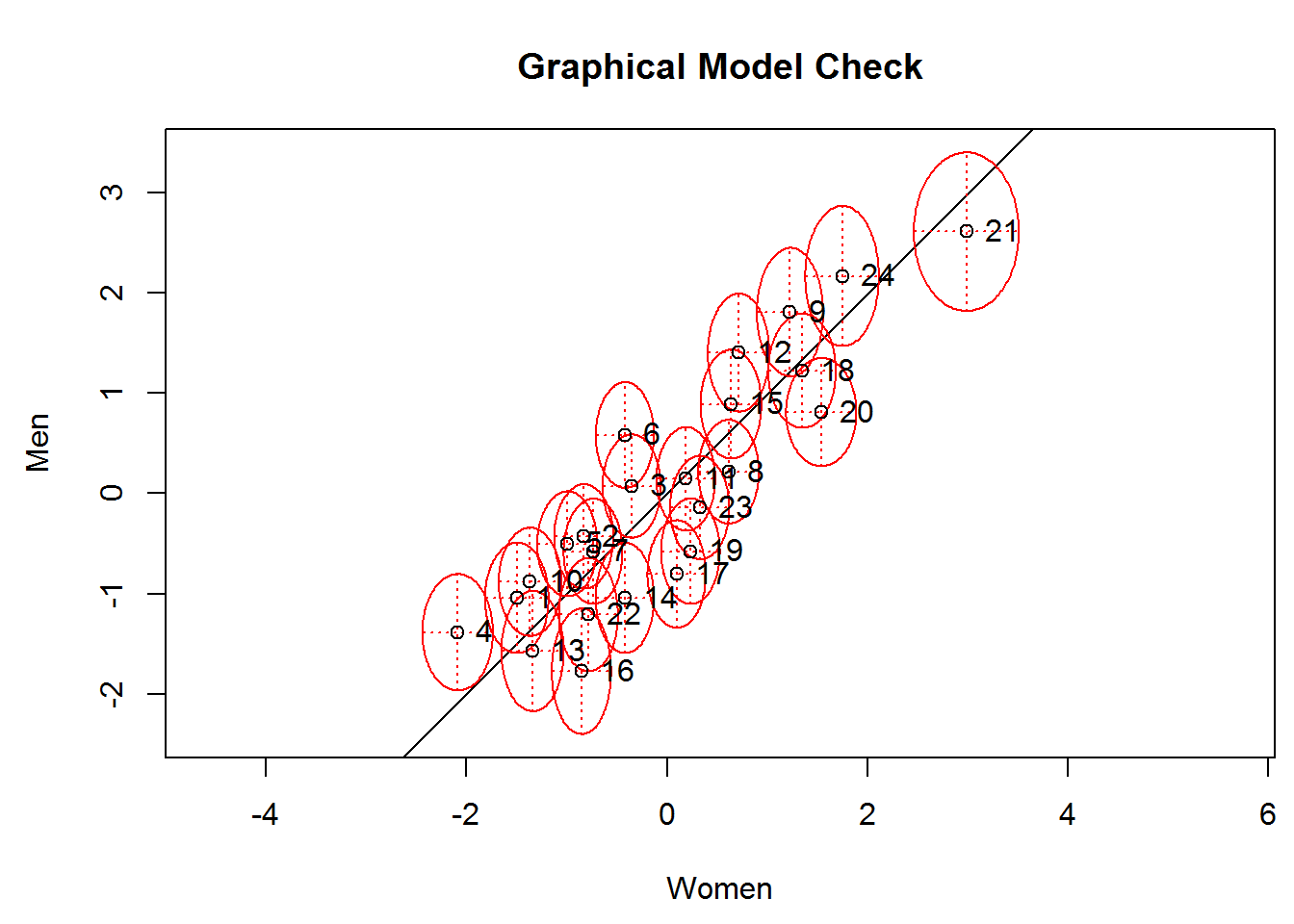
lrt_1
#>
#> Andersen LR-test:
#> LR-value: 70.693
#> Chi-square df: 23
#> p-value:  0
Removing bad fitting items should improve fit, and this is indeed the case here if item 6 is removed: The test statistic is smaller now even though still significant.
tmp1 <- RM(dat_1[, -6])
LRtest(tmp1, splitcr = verbal$Gender)
#>
#> Andersen LR-test:
#> LR-value: 59.533
#> Chi-square df: 22
#> p-value:  0
Wald Test
The Wald test is also based on the comparison of two groups; however it is used for individual items. Again, misfit is indicated for item 6 among others. It is interesting to note that the z-statistic is mostly negative for do-items and positive for want-items. Negative values indicate that the item is easier for the second group, namely, men. Thus, it seems easier for men compared to women to “do” or show verbal aggression.
Waldtest(res_rm_1, splitcr = verbal$Gender)
#>
#> Wald test on item level (z-values):
#>
#>                  z-statistic p-value
#> beta S1wantCurse       1.402   0.161
#> beta S1WantScold       1.306   0.192
#> beta S1WantShout       1.408   0.159
#> beta S2WantCurse       2.028   0.043
#> beta S2WantScold       1.595   0.111
#> beta S2WantShout       3.260   0.001
#> beta S3WantCurse       0.518   0.604
#> beta S3WantScold      -1.304   0.192
#> beta S3WantShout       1.579   0.114
#> beta S4WantCurse       1.518   0.129
#> beta S4WantScold      -0.146   0.884
#> beta S4WantShout       2.038   0.042
#> beta S1DoCurse        -0.675   0.500
#> beta S1DoScold        -1.963   0.050
#> beta S1DoShout         0.789   0.430
#> beta S2DoCurse        -2.610   0.009
#> beta S2DoScold        -2.898   0.004
#> beta S2DoShout        -0.368   0.713
#> beta S3DoCurse        -2.645   0.008
#> beta S3DoScold        -2.218   0.027
#> beta S3DoShout        -0.773   0.440
#> beta S4DoCurse        -1.315   0.189
#> beta S4DoScold        -1.547   0.122
#> beta S4DoShout         1.046   0.295
Infit and Outfit
Infit and outfit statistics are not based on the comparison of groups, but on residuals. Descriptively, the MSQ values should be, for instance, within the range from 0.7 to 1.3 (Wright & Linacre, 1994). A t-test is also reported for infit and outfit, and the t-value should conventionally be within the range from -1.96 to +1.96. Here, the previously flagged item 6 performs quite good, but other items do not, for example item 14 (S1DoScold). The eRm package also provides a plot of the infit t-values, called a Pathway Map, which is also available for persons instead of items (i.e., plotPWmap(res_rm_1, pmap = TRUE, imap = FALSE)).
# To calculate infit/outfit via itemfit(), the person parameters have to be
# estimated first
pp_ml_1 <- person.parameter(res_rm_1)
itemfit(pp_ml_1)
#>
#> Itemfit Statistics:
#>                Chisq  df p-value Outfit MSQ Infit MSQ Outfit t Infit t
#> S1wantCurse  333.752 306   0.132      1.087     0.973     0.58   -0.36
#> S1WantScold  285.433 306   0.795      0.930     0.959    -0.58   -0.69
#> S1WantShout  303.008 306   0.538      0.987     0.981    -0.09   -0.33
#> S2WantCurse  231.914 306   0.999      0.755     0.976    -1.18   -0.25
#> S2WantScold  274.211 306   0.904      0.893     0.950    -0.85   -0.83
#> S2WantShout  296.628 306   0.639      0.966     1.001    -0.30    0.04
#> S3WantCurse  370.936 306   0.006      1.208     1.138     1.73    2.27
#> S3WantScold  267.323 306   0.946      0.871     0.956    -1.10   -0.72
#> S3WantShout  399.960 306   0.000      1.303     1.097     1.58    1.19
#> S4WantCurse  298.519 306   0.609      0.972     1.051    -0.14    0.77
#> S4WantScold  297.046 306   0.633      0.968     0.929    -0.27   -1.27
#> S4WantShout  366.629 306   0.010      1.194     1.082     1.35    1.21
#> S1DoCurse    256.352 306   0.982      0.835     0.895    -1.04   -1.53
#> S1DoScold    226.531 306   1.000      0.738     0.837    -2.59   -3.01
#> S1DoShout    294.109 306   0.677      0.958     0.956    -0.29   -0.68
#> S2DoCurse    301.914 306   0.555      0.983     0.951    -0.08   -0.77
#> S2DoScold    246.872 306   0.994      0.804     0.891    -2.01   -2.02
#> S2DoShout    267.965 306   0.943      0.873     0.910    -0.69   -1.14
#> S3DoCurse    345.909 306   0.058      1.127     1.069     1.21    1.23
#> S3DoScold    263.468 306   0.962      0.858     1.006    -0.77    0.10
#> S3DoShout   1001.107 306   0.000      3.261     0.986     3.70   -0.04
#> S4DoCurse    285.345 306   0.796      0.929     0.970    -0.54   -0.49
#> S4DoScold    289.620 306   0.741      0.943     0.996    -0.50   -0.05
#> S4DoShout    312.841 306   0.382      1.019     1.035     0.16    0.38

plotPWmap(res_rm_1)
DIF
Herein, differential item functioning (DIF) or item bias or measurement invariance is treated as a topic within Model Fit, but it could also be treated as a topic of its own given the high relevance in the IRT literature.
Above, we already compared item parameters across groups from a fit perspective. However, if the groups are the focal and the reference group, these procedures can also be interpreted from a DIF perspective. Thus, the Wald test indicated that item 6 showed DIF, namely, uniform DIF.
Mantel-Haenszel
The Mantel-Haenszel method is a non-parametric approach to DIF. Herein, again item 6 is flagged having significant DIF (p = .002) with a large effect size of \(\Delta_{MH}\)=-2.49. The negative effect size indicates that the item is harder for the focal group, namely, men, mirroring the results from above. The plot gives a compact summary across all items.
tmp1 <- difMH(dat_1, group = verbal$Gender, focal.name = 1)
tmp1
#>
#> Detection of Differential Item Functioning using Mantel-Haenszel method
#> with continuity correction and without item purification
#>
#> Results based on asymptotic inference
#>
#> Matching variable: test score
#>
#> No set of anchor items was provided
#>
#> No p-value adjustment for multiple comparisons
#>
#> Mantel-Haenszel Chi-square statistic:
#>
#>             Stat.  P-value
#> S1wantCurse 1.7076 0.1913
#> S1WantScold 2.1486 0.1427
#> S1WantShout 0.9926 0.3191
#> S2WantCurse 1.9302 0.1647
#> S2WantScold 2.9540 0.0857  .
#> S2WantShout 9.6032 0.0019  **
#> S3WantCurse 0.0013 0.9711
#> S3WantScold 0.6752 0.4112
#> S3WantShout 0.8185 0.3656
#> S4WantCurse 1.6292 0.2018
#> S4WantScold 0.0152 0.9020
#> S4WantShout 4.1188 0.0424  *
#> S1DoCurse   0.1324 0.7160
#> S1DoScold   2.7501 0.0972  .
#> S1DoShout   0.0683 0.7938
#> S2DoCurse   6.3029 0.0121  *
#> S2DoScold   6.8395 0.0089  **
#> S2DoShout   0.2170 0.6414
#> S3DoCurse   5.7817 0.0162  *
#> S3DoScold   3.8880 0.0486  *
#> S3DoShout   0.2989 0.5846
#> S4DoCurse   1.1220 0.2895
#> S4DoScold   1.4491 0.2287
#> S4DoShout   0.8390 0.3597
#>
#> Signif. codes: 0 '***' 0.001 '**' 0.01 '*' 0.05 '.' 0.1 ' ' 1
#>
#> Detection threshold: 3.8415 (significance level: 0.05)
#>
#> Items detected as DIF items:
#>
#>  S2WantShout
#>  S4WantShout
#>  S2DoCurse
#>  S2DoScold
#>  S3DoCurse
#>  S3DoScold
#>
#>
#> Effect size (ETS Delta scale):
#>
#> Effect size code:
#>  'A': negligible effect
#>  'B': moderate effect
#>  'C': large effect
#>
#>             alphaMH deltaMH
#> S1wantCurse  1.7005 -1.2476 B
#> S1WantScold  1.7702 -1.3420 B
#> S1WantShout  1.4481 -0.8701 A
#> S2WantCurse  1.9395 -1.5567 C
#> S2WantScold  1.9799 -1.6052 C
#> S2WantShout  2.8804 -2.4861 C
#> S3WantCurse  0.9439  0.1358 A
#> S3WantScold  0.7194  0.7741 A
#> S3WantShout  1.5281 -0.9965 A
#> S4WantCurse  1.6849 -1.2260 B
#> S4WantScold  1.0901 -0.2028 A
#> S4WantShout  2.3458 -2.0036 C
#> S1DoCurse    0.7967  0.5340 A
#> S1DoScold    0.4995  1.6313 C
#> S1DoShout    1.1765 -0.3821 A
#> S2DoCurse    0.3209  2.6709 C
#> S2DoScold    0.3746  2.3072 C
#> S2DoShout    0.7931  0.5447 A
#> S3DoCurse    0.4616  1.8165 C
#> S3DoScold    0.4727  1.7606 C
#> S3DoShout    0.6373  1.0585 B
#> S4DoCurse    0.6444  1.0327 B
#> S4DoScold    0.6385  1.0541 B
#> S4DoShout    1.6053 -1.1123 B
#>
#> Effect size codes: 0 'A' 1.0 'B' 1.5 'C'
#>  (for absolute values of 'deltaMH')
#>
#> Output was not captured!

plot(tmp1)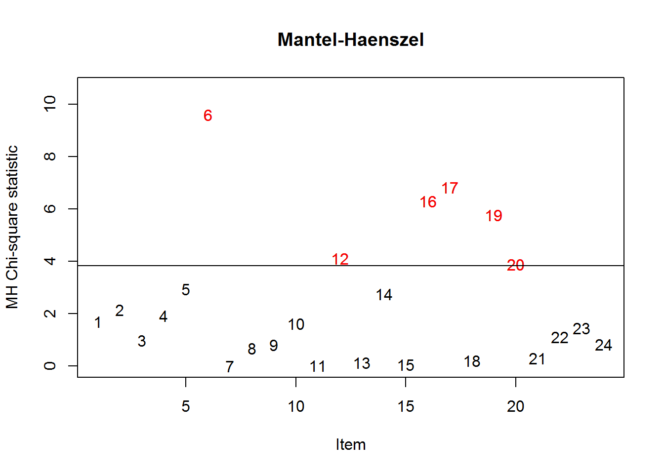
#> The plot was not captured!Lord’s Chi-Square-Test
Lord’s \(\chi^2\)-Test allows to test for non-uniform (crossing) DIF, because a 2PL (or even 3PL) model is estimated in each group rather than a Rasch model, which was used for the Wald test.
Here, item 6 has still a relatively high \(\chi^2\)-value but it is non-significant (p = .075). The ICCs indicate that item 6 is a little bit harder for men and also a little bit less discriminating (uniform and non-uniform DIF)—but non-significant.
tmp1 <- difLord(dat_1, group = verbal$Gender, focal.name = 1, model = "2PL")
# tmp1 <- difLord(dat_1, group = verbal$Gender, focal.name = 1, model = "1PL", discr = NULL)
tmp1
#>
#> Detection of Differential Item Functioning using Lord's method
#> with 2PL model and without item purification
#>
#> Engine 'ltm' for item parameter estimation
#>
#> No set of anchor items was provided
#>
#> No p-value adjustment for multiple comparisons
#>
#> Lord's chi-square statistic:
#>
#>             Stat.  P-value
#> S1wantCurse 1.3458 0.5102
#> S1WantScold 2.3185 0.3137
#> S1WantShout 0.8788 0.6444
#> S2WantCurse 4.5812 0.1012
#> S2WantScold 3.3121 0.1909
#> S2WantShout 5.1932 0.0745  .
#> S3WantCurse 1.1636 0.5589
#> S3WantScold 2.2611 0.3229
#> S3WantShout 1.0015 0.6061
#> S4WantCurse 2.8886 0.2359
#> S4WantScold 0.6412 0.7257
#> S4WantShout 2.1526 0.3409
#> S1DoCurse   1.8026 0.4060
#> S1DoScold   3.7448 0.1538
#> S1DoShout   0.3376 0.8447
#> S2DoCurse   7.6852 0.0214  *
#> S2DoScold   6.9684 0.0307  *
#> S2DoShout   2.7932 0.2474
#> S3DoCurse   5.6040 0.0607  .
#> S3DoScold   5.6378 0.0597  .
#> S3DoShout   0.9704 0.6156
#> S4DoCurse   3.5649 0.1682
#> S4DoScold   4.2514 0.1193
#> S4DoShout   0.4827 0.7856
#>
#> Signif. codes: 0 '***' 0.001 '**' 0.01 '*' 0.05 '.' 0.1 ' ' 1
#>
#> Detection threshold: 5.9915 (significance level: 0.05)
#>
#> Items detected as DIF items:
#>
#>  S2DoCurse
#>  S2DoScold
#>
#> Output was not captured!

plot(tmp1)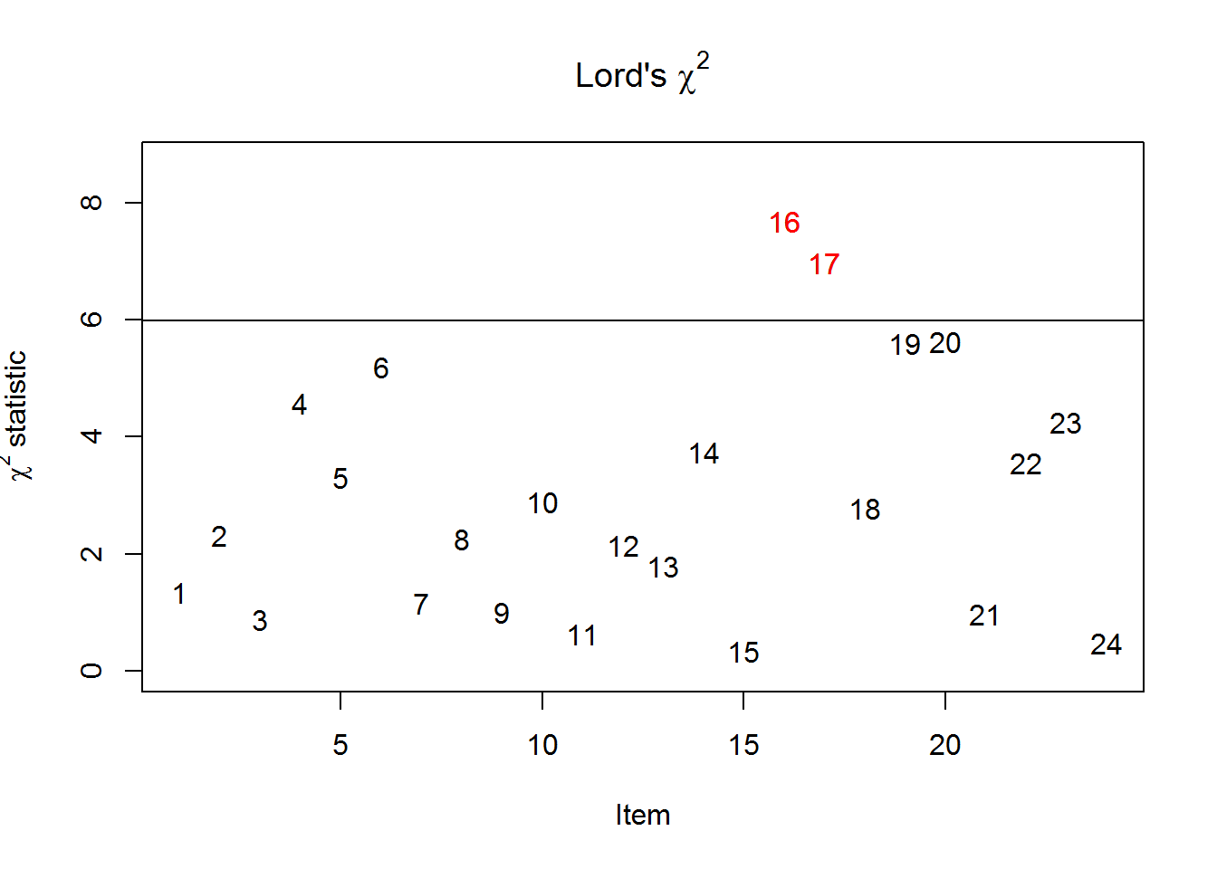
#> The plot was not captured!
plot(tmp1, plot = "itemCurve", item = 6)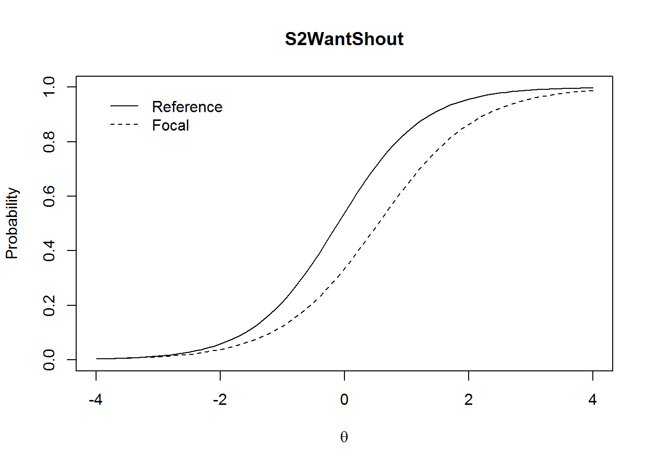
#> The plot was not captured!Person Parameters
An ability parameter for every person can be estimated using different methods, and those will be illustrated and compared in the following.
ML
Maximum likelihood (ML) estimation without further assumptions/information is available in the eRm package. ML estimation does not allow an estimate for persons who solved none or all items. Estimates are calculated via extrapolation for those persons per default (i.e., coef(extrapolated = TRUE)), but this can be disabled.
tmp1 <- person.parameter(res_rm_1)
pp_ml <- coef(tmp1)
MAP and EAP
Maximum a Posteriori (MAP) also known as Empirical Bayes (EB) estimates are available in the ltm package, as well as the closely related Expected a Posteriori (EAP) estimates. Both assume a normal distribution prior for the person parameters.
The extremely high correlation among the estimates indicates that the methods lead to the same conclusions for the present data set, and this will often be the case.
pp_map <- factor.scores(res_rm_2, method = "EB", resp.patterns = dat_1)
pp_eap <- factor.scores(res_rm_2, method = "EAP", resp.patterns = dat_1)
tmp1 <- data.frame(ML = pp_ml, MAP = pp_map$score.dat$z1, EAP = pp_eap$score.dat$z1)
round(cor(tmp1), 4)
#>         ML    MAP    EAP
#> ML  1.0000 0.9950 0.9954
#> MAP 0.9950 1.0000 0.9999
#> EAP 0.9954 0.9999 1.0000
Furthermore, the scatter plot of the ML and the MAP estimates illustrates the effect of the prior. The relationship is linear for intermediate person parameters. However, shrinkage towards 0 is observed for extreme person parameters such that the MAP estimates are less extreme than the ML estimates.
plot(tmp1[, 1:2])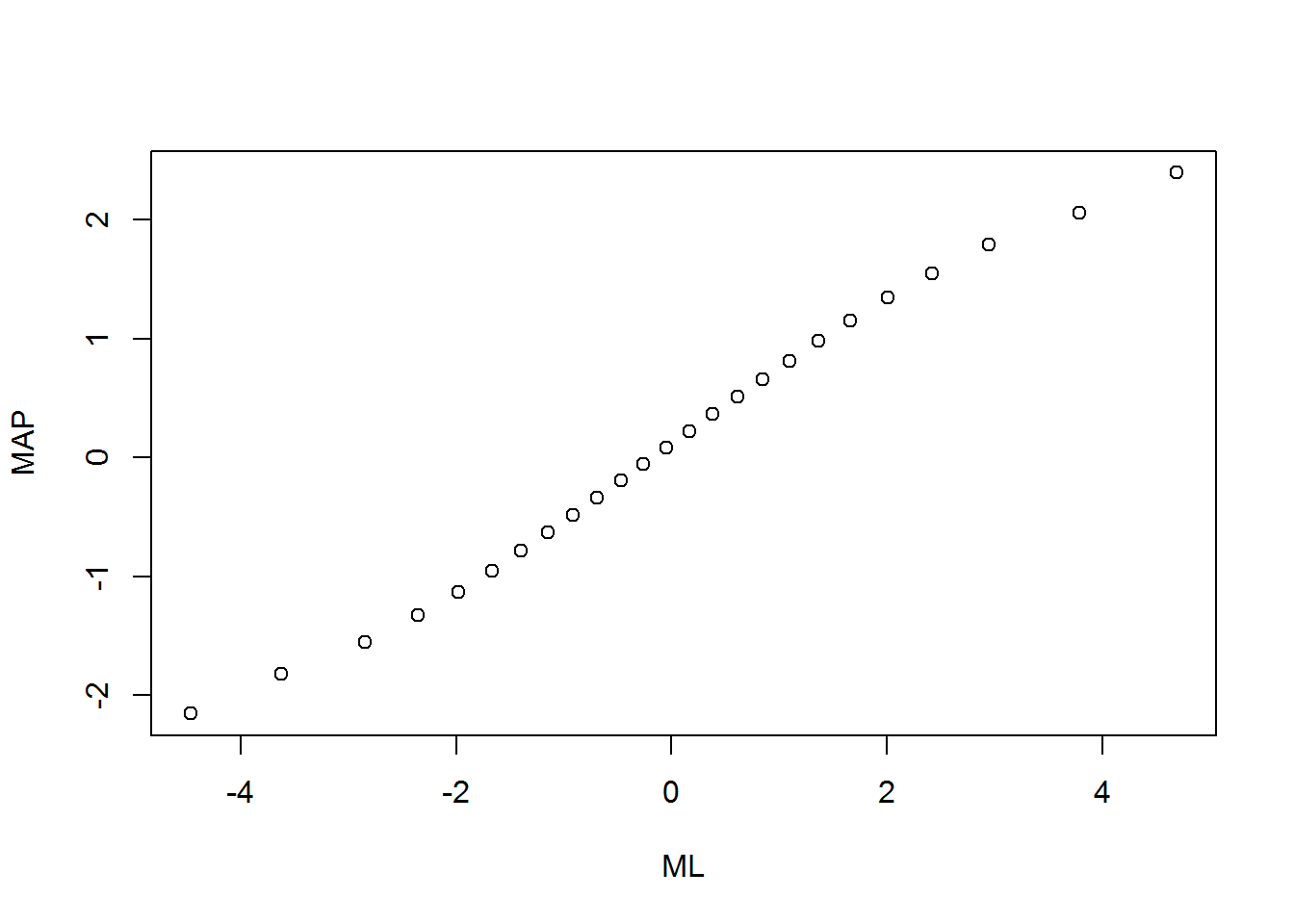
Furthermore, we may compare the estimates for the Rasch and the 2PL model as a supplement to the model comparison from above. Again, the person parameters are almost identical highlighting again that the difference between the two models is not large for the present data set.
pp_2pl <- factor.scores(res_2pl_1, method = "EB", resp.patterns = dat_1)
cor(pp_map$score.dat$z1, pp_2pl$score.dat$z1)
#> [1] 0.9956129
Item and Test Information
Item information curves (IICs) are available in both the eRm (plotINFO()) and ltm (plot(type = "IIC")) package. Those curves are an illustration of the difficulty and discrimination parameters. Therefore, it is expected that maximum information is highest for the items with the highest discrimination parameter (e.g., item 14 S1DoScold). It is interesting to see that the do-items show generally larger discrimination parameters, which is often interpreted as being a closer or better measure of the latent variable.
res_2pl_1
#>
#> Call:
#> ltm(formula = dat_1 ~ z1)
#>
#> Coefficients:
#>              Dffclt  Dscrmn
#> S1wantCurse  -0.913   1.358
#> S1WantScold  -0.409   1.525
#> S1WantShout  -0.078   1.340
#> S2WantCurse  -1.243   1.468
#> S2WantScold  -0.500   1.567
#> S2WantShout  -0.026   1.249
#> S3WantCurse  -0.531   0.880
#> S3WantScold   0.475   1.409
#> S3WantShout   1.455   0.912
#> S4WantCurse  -0.906   1.129
#> S4WantScold   0.214   1.588
#> S4WantShout   0.946   0.967
#> S1DoCurse    -0.821   1.666
#> S1DoScold    -0.251   2.272
#> S1DoShout     0.605   1.420
#> S2DoCurse    -0.630   1.475
#> S2DoScold     0.009   1.987
#> S2DoShout     0.968   1.625
#> S3DoCurse     0.164   1.089
#> S3DoScold     1.098   1.342
#> S3DoShout     2.457   1.126
#> S4DoCurse    -0.537   1.363
#> S4DoScold     0.255   1.430
#> S4DoShout     1.592   1.180
#>
#> Log.Lik: -4017.413

plot(res_2pl_1, items =  1:12, type = "IIC", ylim = c(0, 1.3))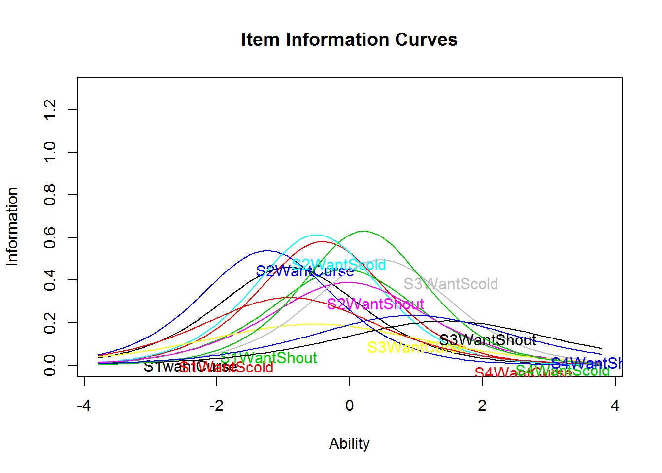
plot(res_2pl_1, items = 13:24, type = "IIC", ylim = c(0, 1.3))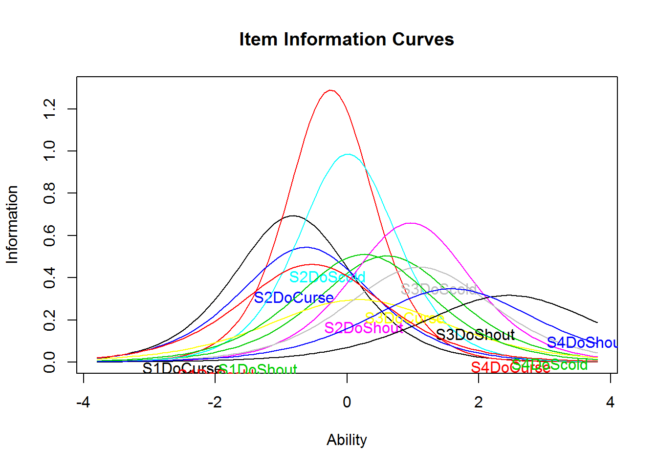
plot(res_2pl_1, items = 0, type = "IIC")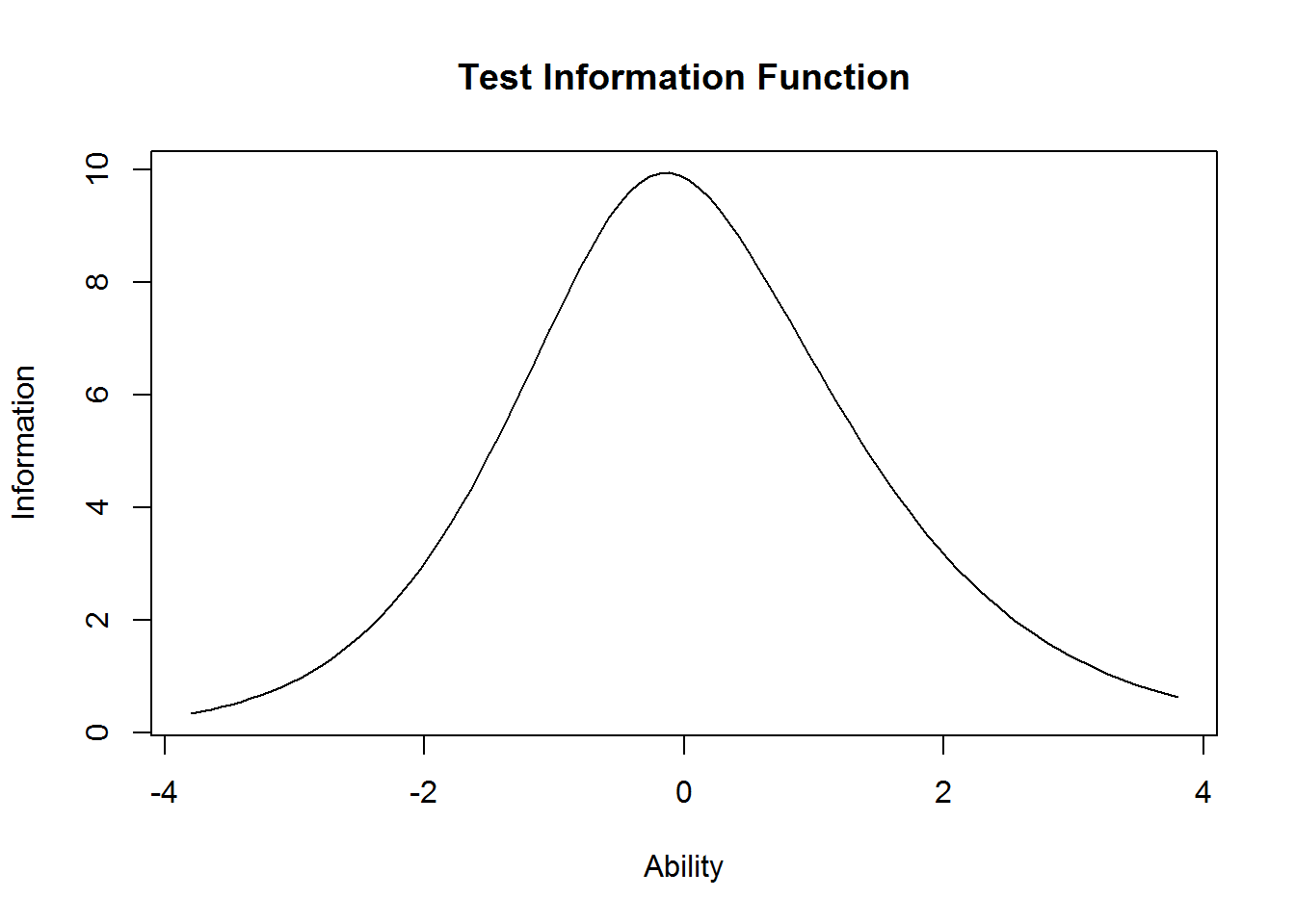
References
Andersen, E. B. (1973). A goodness of fit test for the Rasch model. Psychometrika, 38, 123–140. https://doi.org/10.1007/BF02291180
Magis, D., Béland, S., Tuerlinckx, F., & De Boeck, P. (2010). A general framework and an R package for the detection of dichotomous differential item functioning. Behavior Research Methods, 42, 847–862. https://doi.org/10.3758/BRM.42.3.847
Mair, P., & Hatzinger, R. (2007). Extended Rasch modeling: The eRm package for the application of IRT models in R. Journal of Statistical Software, 20(9), 1–20. https://doi.org/10.18637/jss.v020.i09
Rizopoulos, D. (2006). ltm: An R package for latent variable modelling and item response theory analyses. Journal of Statistical Software, 17(5), 1–25. Retrieved from http://www.jstatsoft.org/v17/i05/
Wright, B. D., & Linacre, J. M. (1994). Reasonable mean-square fit values. Rasch Measurement Transactions, 8, 370. Retrieved from https://www.rasch.org/rmt/rmt83b.htm