- Set Up
- Data Set: Diamonds
- Separating Testing and Training Data: rsample
- Data Pre-Processing and Feature Engineering: recipes
- Defining and Fitting Models: parsnip
- Summarizing Fitted Models: broom
- Evaluating Model Performance: yardstick
- Tuning Model Parameters: tune and dials
- Summary
- Further Resources
- Session Info
- Updates
caret is a well known R package for machine learning, which includes almost everything from data pre-processing to cross-validation. The unofficial successor of caret is tidymodels, which has a modular approach meaning that specific, smaller packages are designed to work hand in hand. Thus, tidymodels is to modeling what the tidyverse is to data wrangling. Herein, I will walk through a machine learning example from start to end and explain how to use the appropriate tidymodels packages at each place.
Set Up
Loading the tidymodels package loads a bunch of packages for modeling and also a few others from the tidyverse like ggplot2 and dplyr.
library("conflicted")
library("tidymodels")
#> -- Attaching packages ------------------------------------------------ tidymodels 0.1.0 --
#> v broom     0.5.5      v recipes   0.1.10
#> v dials     0.0.6      v rsample   0.0.6
#> v dplyr     0.8.5      v tibble    3.0.0
#> v ggplot2   3.3.0      v tune      0.1.0
#> v infer     0.5.1      v workflows 0.1.1
#> v parsnip   0.0.5      v yardstick 0.0.6
#> v purrr     0.3.3

# Additional packages for dataviz etc.
library("ggrepel")     # for geom_label_repel()
library("corrplot")    # for corrplot()
#> corrplot 0.84 loaded

conflict_prefer("filter", "dplyr")
#> [conflicted] Will prefer dplyr::filter over any other package

ggplot2::theme_set(theme_light())
Data Set: Diamonds
With ggplot2 comes the diamonds data set, which has information on the size and quality of diamonds. Herein, we’ll use these features to predict the price of a diamond.
data("diamonds")
diamonds %>%
    sample_n(2000) %>%
    mutate_if(is.factor, as.numeric) %>%
    select(price, everything()) %>%
    cor %>%
    {.[order(abs(.[, 1]), decreasing = TRUE),
       order(abs(.[, 1]), decreasing = TRUE)]} %>%
    corrplot(method = "number", type = "upper", mar = c(0, 0, 1.5, 0),
             title = "Correlations between price and various features of diamonds")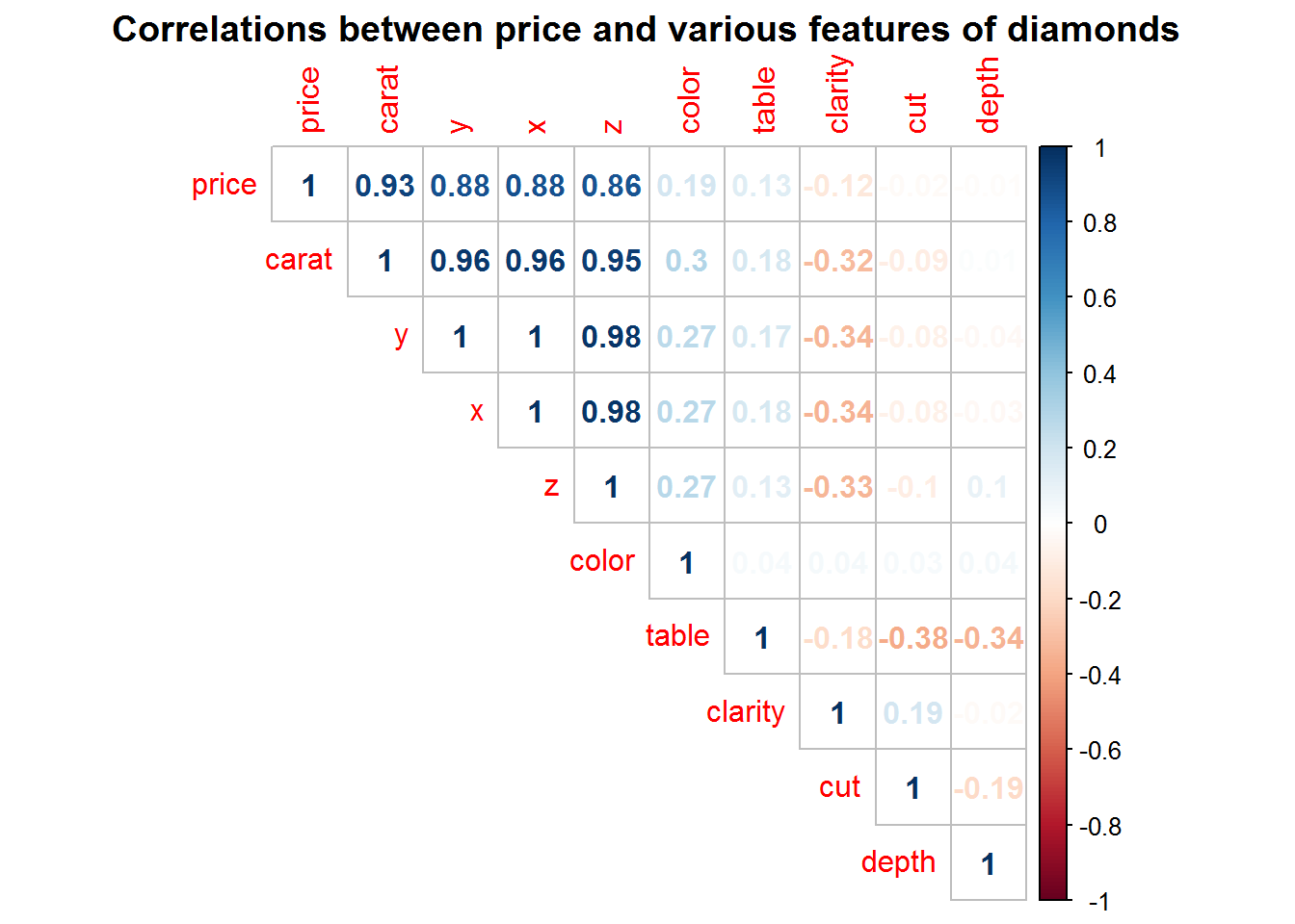
Separating Testing and Training Data: rsample
First of all, we want to extract a data set for testing the predictions in the end. We’ll only use a small proportion for training (only to speed things up a little). Furthermore, the training data set will be prepared for 3-fold cross-validation (using three here to speed things up). All this is accomplished using the rsample package:
set.seed(1243)

dia_split <- initial_split(diamonds, prop = .1, strata = price)

dia_train <- training(dia_split)
dia_test  <- testing(dia_split)

dim(dia_train)
#> [1] 5395   10
dim(dia_test)
#> [1] 48545    10

dia_vfold <- vfold_cv(dia_train, v = 3, repeats = 1, strata = price)
dia_vfold %>%
  mutate(df_ana = map(splits, analysis),
         df_ass = map(splits, assessment))
#> #  3-fold cross-validation using stratification
#> # A tibble: 3 x 4
#>   splits              id    df_ana                df_ass
#> * <named list>        <chr> <named list>          <named list>
#> 1 <split [3.6K/1.8K]> Fold1 <tibble [3,596 x 10]> <tibble [1,799 x 10]>
#> 2 <split [3.6K/1.8K]> Fold2 <tibble [3,596 x 10]> <tibble [1,799 x 10]>
#> 3 <split [3.6K/1.8K]> Fold3 <tibble [3,598 x 10]> <tibble [1,797 x 10]>
Data Pre-Processing and Feature Engineering: recipes
The recipes package can be used to prepare a data set (for modeling) using different step_*() functions.
For example, the plot below indicates that there may be a nonlinear relationship between price and carat, and I want to address that using higher-order terms.
qplot(carat, price, data = dia_train) +
    scale_y_continuous(trans = log_trans(), labels = function(x) round(x, -2)) +
    geom_smooth(method = "lm", formula = "y ~ poly(x, 4)") +
    labs(title = "Nonlinear relationship between price and carat of diamonds",
         subtitle = "The degree of the polynomial is a potential tuning parameter")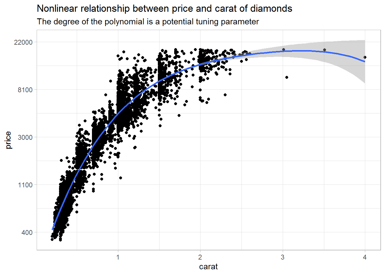
The recipe() takes a formula and a data set, and then the different steps are added using the appropriate step_*() functions.
The recipes package comes with a ton of useful step functions (see, e.g., vignette("Simple_Example", package = "recipes")).
Herein, I want to log transform price (step_log()), I want to center and scale all numeric predictors (step_normalize()), and the categorical predictors should be dummy coded (step_dummy()).
Furthermore, a quadratic effect of carat is added using step_poly().
dia_rec <-
    recipe(price ~ ., data = dia_train) %>%
    step_log(all_outcomes()) %>%
    step_normalize(all_predictors(), -all_nominal()) %>%
    step_dummy(all_nominal()) %>%
    step_poly(carat, degree = 2)

prep(dia_rec)
#> Data Recipe
#>
#> Inputs:
#>
#>       role #variables
#>    outcome          1
#>  predictor          9
#>
#> Training data contained 5395 data points and no missing data.
#>
#> Operations:
#>
#> Log transformation on price [trained]
#> Centering and scaling for carat, depth, table, x, y, z [trained]
#> Dummy variables from cut, color, clarity [trained]
#> Orthogonal polynomials on carat [trained]
Calling prep() on a recipe applies all the steps.
You can now call juice() to extract the transformed data set or call bake() on a new data set.
# Note the linear and quadratic term for carat and the dummies for e.g. color
dia_juiced <- juice(prep(dia_rec))
dim(dia_juiced)
#> [1] 5395   25
names(dia_juiced)
#>  [1] "depth"        "table"        "x"            "y"            "z"
#>  [6] "price"        "cut_1"        "cut_2"        "cut_3"        "cut_4"
#> [11] "color_1"      "color_2"      "color_3"      "color_4"      "color_5"
#> [16] "color_6"      "clarity_1"    "clarity_2"    "clarity_3"    "clarity_4"
#> [21] "clarity_5"    "clarity_6"    "clarity_7"    "carat_poly_1" "carat_poly_2"
Defining and Fitting Models: parsnip
The parsnip package has wrappers around many1 popular machine learning algorithms, and you can fit them using a unified interface. This is extremely helpful, since you have to remember only one rather then dozens of interfaces.
The models are separated into two modes/categories, namely, regression and classification (set_mode()).
The model is defined using a function specific to each algorithm (e.g., linear_reg(), rand_forest()).
Finally, the backend/engine/implementation is selected using set_engine().
Herein, I will start with a basic linear regression model as implemented in stats::lm().
lm_model <-
    linear_reg() %>%
    set_mode("regression") %>%
    set_engine("lm")
Furthermore, take the example of a random forest model.
This could be fit using packages ranger or randomForest.
Both have different interfaces (e.g., argument ntree vs. num.trees), and parsnip removes the hassle of remembering both interfaces.
More general arguments pertaining to the algorithm are specified in the algorithm function (e.g., rand_forest()).
Arguments specific to the engine are specified in set_engine().
rand_forest(mtry = 3, trees = 500, min_n = 5) %>%
    set_mode("regression") %>%
    set_engine("ranger", importance = "impurity_corrected")
Finally, we can fit() the model.
lm_fit1 <- fit(lm_model, price ~ ., dia_juiced)
lm_fit1
#> parsnip model object
#>
#> Fit time:  20ms
#>
#> Call:
#> stats::lm(formula = formula, data = data)
#>
#> Coefficients:
#>  (Intercept)         depth         table             x             y
#>     7.711965      0.010871      0.005889      0.251155      0.054422
#>            z         cut_1         cut_2         cut_3         cut_4
#>     0.054196      0.106701     -0.026356      0.024207     -0.006191
#>      color_1       color_2       color_3       color_4       color_5
#>    -0.455831     -0.084108     -0.004810      0.009725     -0.005591
#>      color_6     clarity_1     clarity_2     clarity_3     clarity_4
#>    -0.009730      0.860961     -0.242698      0.132234     -0.052903
#>    clarity_5     clarity_6     clarity_7  carat_poly_1  carat_poly_2
#>     0.028996      0.002403      0.022235     51.663971    -17.508316
You can use fit() with a formula (e.g., price ~ .) or by specifying x and y.
In both cases, I recommend keeping only the variables you need when preparing the data set, since this will prevent forgetting the new variable d when using y ~ a + b + c.
Unnecessary variables can easily be dropped in the recipe using step_rm().
Summarizing Fitted Models: broom
Many models have implemented summary() or coef() methods.
However, the output of these is usually not in a tidy format, and the broom package has the aim to resolve this issue.
glance() gives us information about the whole model.
Here, R squared is pretty high and the RMSE equals 0.154.
glance(lm_fit1$fit)
#> # A tibble: 1 x 11
#>   r.squared adj.r.squared sigma statistic p.value    df logLik    AIC    BIC deviance
#>       <dbl>         <dbl> <dbl>     <dbl>   <dbl> <int>  <dbl>  <dbl>  <dbl>    <dbl>
#> 1     0.977         0.977 0.154     9607.       0    25  2457. -4863. -4691.     127.
#> # ... with 1 more variable: df.residual <int>
tidy() gives us information about the model parameters, and we see that we have a significant quadratic effect of carat.
tidy(lm_fit1) %>%
  arrange(desc(abs(statistic)))
#> # A tibble: 25 x 5
#>    term         estimate std.error statistic  p.value
#>    <chr>           <dbl>     <dbl>     <dbl>    <dbl>
#>  1 (Intercept)    7.71     0.00431   1790.   0.
#>  2 carat_poly_2 -17.5      0.259      -67.7  0.
#>  3 clarity_1      0.861    0.0135      64.0  0.
#>  4 color_1       -0.456    0.00738    -61.8  0.
#>  5 carat_poly_1  51.7      1.10        47.0  0.
#>  6 clarity_2     -0.243    0.0127     -19.2  3.63e-79
#>  7 color_2       -0.0841   0.00665    -12.7  3.50e-36
#>  8 clarity_3      0.132    0.0107      12.3  2.51e-34
#>  9 cut_1          0.107    0.00997     10.7  1.88e-26
#> 10 clarity_4     -0.0529   0.00839     -6.30 3.15e-10
#> # ... with 15 more rows
Finally, augment() can be used to get model predictions, residuals, etc.
lm_predicted <- augment(lm_fit1$fit, data = dia_juiced) %>%
    rowid_to_column()
select(lm_predicted, rowid, price, .fitted:.std.resid)
#> # A tibble: 5,395 x 9
#>    rowid price .fitted .se.fit  .resid    .hat .sigma   .cooksd .std.resid
#>    <int> <dbl>   <dbl>   <dbl>   <dbl>   <dbl>  <dbl>     <dbl>      <dbl>
#>  1     1  5.83    5.90 0.0133  -0.0769 0.00744  0.154 0.0000755     -0.502
#>  2     2  5.84    5.80 0.0110   0.0472 0.00507  0.154 0.0000193      0.307
#>  3     3  5.86    5.89 0.0138  -0.0286 0.00801  0.154 0.0000112     -0.187
#>  4     4  5.88    6.24 0.00988 -0.360  0.00413  0.154 0.000910      -2.34
#>  5     5  6.00    6.24 0.0104  -0.244  0.00458  0.154 0.000467      -1.59
#>  6     6  6.00    6.06 0.0100  -0.0615 0.00427  0.154 0.0000275     -0.401
#>  7     7  6.00    6.10 0.0111  -0.0999 0.00520  0.154 0.0000887     -0.651
#>  8     8  6.00    6.06 0.0104  -0.0566 0.00459  0.154 0.0000251     -0.369
#>  9     9  6.00    6.22 0.00895 -0.216  0.00339  0.154 0.000270      -1.41
#> 10    10  6.32    6.55 0.00872 -0.233  0.00321  0.154 0.000297      -1.52
#> # ... with 5,385 more rows
A plot of the predicted vs. actual prices shows small residuals with a few outliers, which are not well explained by the model.
ggplot(lm_predicted, aes(.fitted, price)) +
    geom_point(alpha = .2) +
    ggrepel::geom_label_repel(aes(label = rowid),
                              data = filter(lm_predicted, abs(.resid) > 2)) +
    labs(title = "Actual vs. Predicted Price of Diamonds")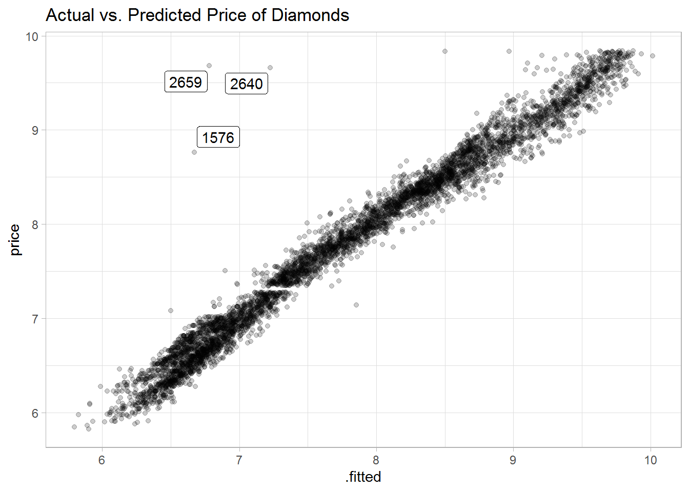
Evaluating Model Performance: yardstick
We already saw performance measures RMSE and R squared in the output of glance() above.
The yardstick package is specifically designed for such measures for both numeric and categorical outcomes, and it plays well with grouped predictions (e.g., from cross-validation).
Let’s use rsample, parsnip, and yardstick for cross-validation to get a more accurate estimation of RMSE.
In the following pipeline, the model is fit() separately to the three analysis data sets, and then the fitted models are used to predict() on the three corresponding assessment data sets (i.e., 3-fold cross-validation).
Before that, analysis() and assessment() are used to extract the respective folds from dia_vfold.
Furthermore, the recipe dia_rec is prepped (i.e., trained) using the analysis data of each fold, and this prepped recipe is then applied to the assessment data of each fold using bake().
Preparing the recipe separately for each fold (rather than once for the whole training data set dia_train) guards against data leakage.
The code in the following chunk makes use of list columns to store all information about the three folds in a single tibble lm_fit2, and a combination of dplyr::mutate() and purrr::map() is used to “loop” across the three rows of the tibble.
# How does dia_vfold look?
dia_vfold
#> #  3-fold cross-validation using stratification
#> # A tibble: 3 x 2
#>   splits              id
#>   <named list>        <chr>
#> 1 <split [3.6K/1.8K]> Fold1
#> 2 <split [3.6K/1.8K]> Fold2
#> 3 <split [3.6K/1.8K]> Fold3

# Extract analysis/training and assessment/testing data
lm_fit2 <- mutate(dia_vfold,
                  df_ana = map (splits,  analysis),
                  df_ass = map (splits,  assessment))
lm_fit2
#> #  3-fold cross-validation using stratification
#> # A tibble: 3 x 4
#>   splits              id    df_ana                df_ass
#> * <named list>        <chr> <named list>          <named list>
#> 1 <split [3.6K/1.8K]> Fold1 <tibble [3,596 x 10]> <tibble [1,799 x 10]>
#> 2 <split [3.6K/1.8K]> Fold2 <tibble [3,596 x 10]> <tibble [1,799 x 10]>
#> 3 <split [3.6K/1.8K]> Fold3 <tibble [3,598 x 10]> <tibble [1,797 x 10]>

lm_fit2 <-
    lm_fit2 %>%
    # prep, juice, bake
    mutate(
        recipe = map (df_ana, ~prep(dia_rec, training = .x)),
        df_ana = map (recipe,  juice),
        df_ass = map2(recipe,
                      df_ass, ~bake(.x, new_data = .y))) %>%
    # fit
    mutate(
        model_fit  = map(df_ana, ~fit(lm_model, price ~ ., data = .x))) %>%
    # predict
    mutate(
        model_pred = map2(model_fit, df_ass, ~predict(.x, new_data = .y)))

select(lm_fit2, id, recipe:model_pred)
#> # A tibble: 3 x 4
#>   id    recipe       model_fit    model_pred
#>   <chr> <named list> <named list> <named list>
#> 1 Fold1 <recipe>     <fit[+]>     <tibble [1,799 x 1]>
#> 2 Fold2 <recipe>     <fit[+]>     <tibble [1,799 x 1]>
#> 3 Fold3 <recipe>     <fit[+]>     <tibble [1,797 x 1]>
Note that the cross-validation code above is a bit lengthy—for didactic purposes.
Wrapper functions (e.g., from the tune package) would lead to more concise code: fit_resamples() could be used here (without tuning), or tune_grid() and tune_bayes() (see below).
Now, we can extract the actual prices price from the assessment data and compare them to the predicted prices .pred.
Then, the yardstick package comes into play: The function metrics() calculates three different metrics for numeric outcomes.
Furthermore, it automatically recognizes that lm_preds is grouped by folds and thus calculates the metrics for each fold.
Across the three folds, we see that the RMSE is a little higher and R squared a little smaller compared to above (see output of glance(lm_fit1$fit)).
This is expected, since out-of-sample prediction is harder but also way more useful.
lm_preds <-
    lm_fit2 %>%
    mutate(res = map2(df_ass, model_pred, ~data.frame(price = .x$price,
                                                      .pred = .y$.pred))) %>%
    select(id, res) %>%
    tidyr::unnest(res) %>%
    group_by(id)
lm_preds
#> # A tibble: 5,395 x 3
#> # Groups:   id [3]
#>    id    price .pred
#>    <chr> <dbl> <dbl>
#>  1 Fold1  5.84  5.83
#>  2 Fold1  6.00  6.25
#>  3 Fold1  6.00  6.05
#>  4 Fold1  6.32  6.56
#>  5 Fold1  6.32  6.31
#>  6 Fold1  7.92  7.73
#>  7 Fold1  7.93  7.58
#>  8 Fold1  7.93  7.80
#>  9 Fold1  7.93  7.88
#> 10 Fold1  7.94  7.91
#> # ... with 5,385 more rows

metrics(lm_preds, truth = price, estimate = .pred)
#> # A tibble: 9 x 4
#>   id    .metric .estimator .estimate
#>   <chr> <chr>   <chr>          <dbl>
#> 1 Fold1 rmse    standard       0.168
#> 2 Fold2 rmse    standard       0.147
#> 3 Fold3 rmse    standard       0.298
#> 4 Fold1 rsq     standard       0.973
#> 5 Fold2 rsq     standard       0.979
#> 6 Fold3 rsq     standard       0.918
#> 7 Fold1 mae     standard       0.116
#> 8 Fold2 mae     standard       0.115
#> 9 Fold3 mae     standard       0.110
Note that metrics() has default measures for numeric and categorical outcomes, and here RMSE, R squared, and the mean absolute difference (MAE) are returned.
You could also use one metric directly like rmse() or define a custom set of metrics via metric_set().
Tuning Model Parameters: tune and dials
Let’s get a little bit more involved and do some hyperparameter tuning. We turn to a different model, namely, a random forest model.
The tune package has functions for doing the actual tuning (e.g., via grid search), while all the parameters and their defaults (e.g., mtry(), neighbors()) are implemented in dials.
Thus, the two packages can almost only be used in combination.
Preparing a parsnip Model for Tuning
First, I want to tune the mtry parameter of a random forest model.
Thus, the model is defined using parsnip as above.
However, rather than using a default value (i.e., mtry = NULL) or one specific value (i.e., mtry = 3), we use tune() as a placeholder and let cross-validation decide on the best value for mtry later on.
As the output indicates, the default minimum of mtry is 1 and the maximum depends on the data.
rf_model <-
    rand_forest(mtry = tune()) %>%
    set_mode("regression") %>%
    set_engine("ranger")

parameters(rf_model)
#> Collection of 1 parameters for tuning
#>
#>    id parameter type object class
#>  mtry           mtry    nparam[?]
#>
#> Model parameters needing finalization:
#>    # Randomly Selected Predictors ('mtry')
#>
#> See `?dials::finalize` or `?dials::update.parameters` for more information.
mtry()
#> # Randomly Selected Predictors  (quantitative)
#> Range: [1, ?]
Thus, this model is not yet ready for fitting.
You can either specify the maximum for mtry yourself using update(), or you can use finalize() to let the data decide on the maximum.
rf_model %>%
    parameters() %>%
    update(mtry = mtry(c(1L, 5L)))
#> Collection of 1 parameters for tuning
#>
#>    id parameter type object class
#>  mtry           mtry    nparam[+]

rf_model %>%
    parameters() %>%
    # Here, the maximum of mtry equals the number of predictors, i.e., 24.
    finalize(x = select(juice(prep(dia_rec)), -price)) %>%
    pull("object")
#> [[1]]
#> # Randomly Selected Predictors  (quantitative)
#> Range: [1, 24]
Preparing Data for Tuning: recipes
The second thing I want to tune is the degree of the polynomial for the variable carat. As you saw in the plot above, polynomials up to a degree of four seemed well suited for the data. However, a simpler model might do equally well, and we want to use cross-validation to decide on the degree that works best.
Similar to tuning parameters in a model, certain aspects of a recipe can be tuned.
Let’s define a second recipe and use tune() inside step_poly().
# Note that this recipe cannot be prepped (and juiced), since "degree" is a
# tuning parameter
dia_rec2 <-
    recipe(price ~ ., data = dia_train) %>%
    step_log(all_outcomes()) %>%
    step_normalize(all_predictors(), -all_nominal()) %>%
    step_dummy(all_nominal()) %>%
    step_poly(carat, degree = tune())

dia_rec2 %>%
    parameters() %>%
    pull("object")
#> [[1]]
#> Polynomial Degree  (quantitative)
#> Range: [1, 3]
Combine Everything: workflows
The workflows package is designed to bundle together different parts of a machine learning pipeline like a recipe or a model.
First, let’s create an initial workflow and add the recipe and the random forest model, both of which have a tuning parameter.
rf_wflow <-
    workflow() %>%
    add_model(rf_model) %>%
    add_recipe(dia_rec2)
rf_wflow
#> == Workflow ==============================================================================
#> Preprocessor: Recipe
#> Model: rand_forest()
#>
#> -- Preprocessor --------------------------------------------------------------------------
#> 4 Recipe Steps
#>
#> * step_log()
#> * step_normalize()
#> * step_dummy()
#> * step_poly()
#>
#> -- Model ---------------------------------------------------------------------------------
#> Random Forest Model Specification (regression)
#>
#> Main Arguments:
#>   mtry = tune()
#>
#> Computational engine: ranger
Second, we need to update the parameters in rf_wflow, because the maximum of mtry is not yet known and the maximum of degree should be four (while three is the default).
rf_param <-
    rf_wflow %>%
    parameters() %>%
    update(mtry = mtry(range = c(3L, 5L)),
           degree = degree_int(range = c(2L, 4L)))
rf_param$object
#> [[1]]
#> # Randomly Selected Predictors  (quantitative)
#> Range: [3, 5]
#>
#> [[2]]
#> Polynomial Degree  (quantitative)
#> Range: [2, 4]
Third, we want to use cross-validation for tuning, that is, to select the best combination of the hyperparameters.
Bayesian optimization (see https://tidymodels.github.io/tune/) is recommended for complex tuning problems, and this can be done using tune_bayes().
Herein, however, grid search will suffice. To this end, let’s create a grid of all necessary parameter combinations.
rf_grid <- grid_regular(rf_param, levels = 3)
rf_grid
#> # A tibble: 9 x 2
#>    mtry degree
#>   <int>  <int>
#> 1     3      2
#> 2     4      2
#> 3     5      2
#> 4     3      3
#> 5     4      3
#> 6     5      3
#> 7     3      4
#> 8     4      4
#> 9     5      4
Cross-validation and hyperparameter tuning can involve fitting many models. Herein, for example, we have to fit 3 x 9 models (folds x parameter combinations). To increase speed, we can fit the models in parallel. This is directly supported by the tune package (see https://tidymodels.github.io/tune/).
library("doFuture")
all_cores <- parallel::detectCores(logical = FALSE) - 1

registerDoFuture()
cl <- makeCluster(all_cores)
plan(future::cluster, workers = cl)
Then, we can finally start tuning.
rf_search <- tune_grid(rf_wflow, grid = rf_grid, resamples = dia_vfold,
                       param_info = rf_param)
The results can be examined using autoplot() and show_best():
autoplot(rf_search, metric = "rmse") +
    labs(title = "Results of Grid Search for Two Tuning Parameters of a Random Forest")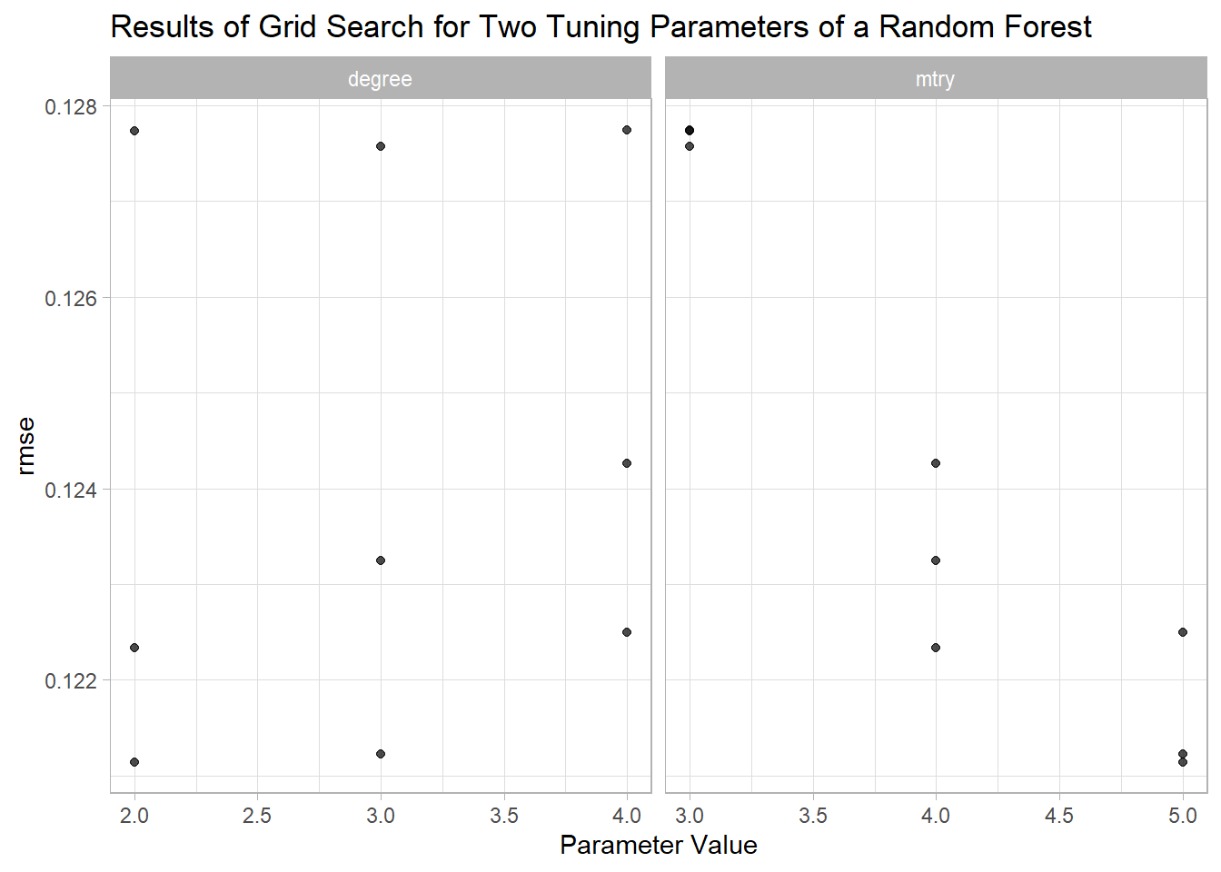
show_best(rf_search, "rmse", n = 9)
#> # A tibble: 9 x 7
#>    mtry degree .metric .estimator  mean     n std_err
#>   <int>  <int> <chr>   <chr>      <dbl> <int>   <dbl>
#> 1     5      2 rmse    standard   0.121     3 0.00498
#> 2     5      3 rmse    standard   0.121     3 0.00454
#> 3     4      2 rmse    standard   0.122     3 0.00463
#> 4     5      4 rmse    standard   0.122     3 0.00471
#> 5     4      3 rmse    standard   0.123     3 0.00469
#> 6     4      4 rmse    standard   0.124     3 0.00496
#> 7     3      3 rmse    standard   0.128     3 0.00502
#> 8     3      2 rmse    standard   0.128     3 0.00569
#> 9     3      4 rmse    standard   0.128     3 0.00501

select_best(rf_search, metric = "rmse")
#> # A tibble: 1 x 2
#>    mtry degree
#>   <int>  <int>
#> 1     5      2

select_by_one_std_err(rf_search, mtry, degree, metric = "rmse")
#> # A tibble: 1 x 9
#>    mtry degree .metric .estimator  mean     n std_err .best .bound
#>   <int>  <int> <chr>   <chr>      <dbl> <int>   <dbl> <dbl>  <dbl>
#> 1     4      2 rmse    standard   0.122     3 0.00463 0.121  0.126
With a cross-validation RMSE of ca. 0.12, the random forest model seems to outperform the linear regression from above. Furthermore, 0.12 is (hopefully) a realistic estimate of the out-of-sample error.
Selecting the Best Model to Make the Final Predictions
We saw above that a quadratic trend was enough to get a good model.
Furthermore, cross-validation revealed that mtry = 4 seems to perform well.
To use this combination of hyperparameters, we fit() the corresponding model (or workflow, more precisely) on the whole training data set dia_train.
rf_param_final <- select_by_one_std_err(rf_search, mtry, degree,
                                        metric = "rmse")

rf_wflow_final <- finalize_workflow(rf_wflow, rf_param_final)

rf_wflow_final_fit <- fit(rf_wflow_final, data = dia_train)
Now, we want to use this to predict() on data never seen before, namely, dia_test.
Unfortunately, predict(rf_wflow_final_fit, new_data = dia_test) does not work in the present case, because the outcome is modified in the recipe via step_log().2
Thus, we need a little workaround:
The prepped recipe is extracted from the workflow, and this can then be used to bake() the testing data.
This baked data set together with the extracted model can then be used for the final predictions.
dia_rec3     <- pull_workflow_prepped_recipe(rf_wflow_final_fit)
rf_final_fit <- pull_workflow_fit(rf_wflow_final_fit)

dia_test$.pred <- predict(rf_final_fit,
                          new_data = bake(dia_rec3, dia_test))$.pred
dia_test$logprice <- log(dia_test$price)

metrics(dia_test, truth = logprice, estimate = .pred)
#> # A tibble: 3 x 3
#>   .metric .estimator .estimate
#>   <chr>   <chr>          <dbl>
#> 1 rmse    standard      0.113
#> 2 rsq     standard      0.988
#> 3 mae     standard      0.0846
As you can see, we get an RMSE of 0.11 on the testing data, which is even slightly better compared to the cross-validation RMSE.
Summary
The tidymodels ecosystem bundles together a set of packages that work hand in hand to solve machine-learning problems from start to end. Together with the data-wrangling facilities in the tidyverse and the plotting tools from ggplot2, this makes for a rich toolbox for every data scientist working with R.
The only thing that is definitely missing in tidymodels is a package for combining different machine learning models (i.e., ensemble/stacking/super learner). We have caretEnsemble for caret, and I am sure they are working on something similar for tidymodels at RStudio. Alex Hayes has a related blog post focusing on tidymodels, for those who can’t wait.
Further Resources
- For further information about each of the tidymodels packages, I recommend the vignettes/articles on the respective package homepage (e.g., https://tidymodels.github.io/recipes/ or https://tidymodels.github.io/tune/).
- Max Kuhn, one of the developer of tidymodels packages, was interviewed on the R podcast and on the DataFramed podcast.
- Max Kuhn is the author of the books Applied Predictive Modeling (with Kjell Johnson) and The caret Package.
- R for Data Science by Hadley Wickham and Garrett Grolemund covers all the basics of data import, transformation, visualization, and modeling using tidyverse and tidymodels packages.
- Variable importance (plots) are provided by the package vip, which works well in combination with tidymodels packages.
- Recipe steps for dealing with unbalanced data are provided by the themis package.
- There are a few more tidymodels packages that I did not cover herein, like infer or tidytext. Read more about these at https://tidymodels.github.io/tidymodels/.
Session Info
sessioninfo::session_info()
#> - Session info -------------------------------------------------------------------------
#>  setting  value
#>  version  R version 3.6.2 (2019-12-12)
#>  os       Windows 10 x64
#>  system   x86_64, mingw32
#>  ui       RTerm
#>  language (EN)
#>  collate  German_Germany.1252
#>  ctype    German_Germany.1252
#>  tz       Europe/Berlin
#>  date     2020-04-07
#>
#> - Packages -----------------------------------------------------------------------------
#>  package       * version     date       lib source
#>  assertthat      0.2.1       2019-03-21 [1] CRAN (R 3.6.2)
#>  backports       1.1.6       2020-04-05 [1] CRAN (R 3.6.2)
#>  base64enc       0.1-3       2015-07-28 [1] CRAN (R 3.6.0)
#>  bayesplot       1.7.1       2019-12-01 [1] CRAN (R 3.6.2)
#>  blogdown        0.18        2020-03-04 [1] CRAN (R 3.6.3)
#>  bookdown        0.18        2020-03-05 [1] CRAN (R 3.6.3)
#>  boot            1.3-23      2019-07-05 [2] CRAN (R 3.6.2)
#>  broom         * 0.5.5       2020-02-29 [1] CRAN (R 3.6.3)
#>  callr           3.4.3       2020-03-28 [1] CRAN (R 3.6.2)
#>  class           7.3-15      2019-01-01 [2] CRAN (R 3.6.2)
#>  cli             2.0.2       2020-02-28 [1] CRAN (R 3.6.3)
#>  codetools       0.2-16      2018-12-24 [2] CRAN (R 3.6.2)
#>  colorspace      1.4-1       2019-03-18 [1] CRAN (R 3.6.1)
#>  colourpicker    1.0         2017-09-27 [1] CRAN (R 3.6.2)
#>  conflicted    * 1.0.4       2019-06-21 [1] CRAN (R 3.6.3)
#>  corrplot      * 0.84        2017-10-16 [1] CRAN (R 3.6.3)
#>  crayon          1.3.4       2017-09-16 [1] CRAN (R 3.6.2)
#>  crosstalk       1.1.0.1     2020-03-13 [1] CRAN (R 3.6.3)
#>  dials         * 0.0.6       2020-04-03 [1] CRAN (R 3.6.2)
#>  DiceDesign      1.8-1       2019-07-31 [1] CRAN (R 3.6.2)
#>  digest          0.6.25      2020-02-23 [1] CRAN (R 3.6.3)
#>  dplyr         * 0.8.5       2020-03-07 [1] CRAN (R 3.6.3)
#>  DT              0.13        2020-03-23 [1] CRAN (R 3.6.3)
#>  dygraphs        1.1.1.6     2018-07-11 [1] CRAN (R 3.6.2)
#>  ellipsis        0.3.0       2019-09-20 [1] CRAN (R 3.6.2)
#>  evaluate        0.14        2019-05-28 [1] CRAN (R 3.6.2)
#>  fansi           0.4.1       2020-01-08 [1] CRAN (R 3.6.2)
#>  farver          2.0.3       2020-01-16 [1] CRAN (R 3.6.2)
#>  fastmap         1.0.1       2019-10-08 [1] CRAN (R 3.6.2)
#>  foreach         1.5.0       2020-03-30 [1] CRAN (R 3.6.2)
#>  furrr           0.1.0       2018-05-16 [1] CRAN (R 3.6.2)
#>  future          1.16.0      2020-01-16 [1] CRAN (R 3.6.2)
#>  generics        0.0.2       2018-11-29 [1] CRAN (R 3.6.2)
#>  ggplot2       * 3.3.0       2020-03-05 [1] CRAN (R 3.6.3)
#>  ggrepel       * 0.8.2       2020-03-08 [1] CRAN (R 3.6.3)
#>  ggridges        0.5.2       2020-01-12 [1] CRAN (R 3.6.2)
#>  globals         0.12.5      2019-12-07 [1] CRAN (R 3.6.1)
#>  glue            1.4.0       2020-04-03 [1] CRAN (R 3.6.2)
#>  gower           0.2.1       2019-05-14 [1] CRAN (R 3.6.1)
#>  GPfit           1.0-8       2019-02-08 [1] CRAN (R 3.6.2)
#>  gridExtra       2.3         2017-09-09 [1] CRAN (R 3.6.2)
#>  gtable          0.3.0       2019-03-25 [1] CRAN (R 3.6.2)
#>  gtools          3.8.2       2020-03-31 [1] CRAN (R 3.6.3)
#>  hardhat         0.1.2       2020-02-28 [1] CRAN (R 3.6.3)
#>  htmltools       0.4.0       2019-10-04 [1] CRAN (R 3.6.2)
#>  htmlwidgets     1.5.1       2019-10-08 [1] CRAN (R 3.6.2)
#>  httpuv          1.5.2       2019-09-11 [1] CRAN (R 3.6.2)
#>  igraph          1.2.5       2020-03-19 [1] CRAN (R 3.6.3)
#>  infer         * 0.5.1       2019-11-19 [1] CRAN (R 3.6.2)
#>  inline          0.3.15      2018-05-18 [1] CRAN (R 3.6.2)
#>  ipred           0.9-9       2019-04-28 [1] CRAN (R 3.6.2)
#>  iterators       1.0.12      2019-07-26 [1] CRAN (R 3.6.2)
#>  janeaustenr     0.1.5       2017-06-10 [1] CRAN (R 3.6.2)
#>  knitr           1.28        2020-02-06 [1] CRAN (R 3.6.2)
#>  labeling        0.3         2014-08-23 [1] CRAN (R 3.6.0)
#>  later           1.0.0       2019-10-04 [1] CRAN (R 3.6.2)
#>  lattice         0.20-38     2018-11-04 [2] CRAN (R 3.6.2)
#>  lava            1.6.7       2020-03-05 [1] CRAN (R 3.6.3)
#>  lhs             1.0.1       2019-02-03 [1] CRAN (R 3.6.2)
#>  lifecycle       0.2.0       2020-03-06 [1] CRAN (R 3.6.3)
#>  listenv         0.8.0       2019-12-05 [1] CRAN (R 3.6.2)
#>  lme4            1.1-21      2019-03-05 [1] CRAN (R 3.6.2)
#>  loo             2.2.0       2019-12-19 [1] CRAN (R 3.6.2)
#>  lubridate       1.7.4       2018-04-11 [1] CRAN (R 3.6.2)
#>  magrittr        1.5         2014-11-22 [1] CRAN (R 3.6.2)
#>  markdown        1.1         2019-08-07 [1] CRAN (R 3.6.2)
#>  MASS            7.3-51.4    2019-03-31 [2] CRAN (R 3.6.2)
#>  Matrix          1.2-18      2019-11-27 [2] CRAN (R 3.6.2)
#>  matrixStats     0.56.0      2020-03-13 [1] CRAN (R 3.6.3)
#>  memoise         1.1.0       2017-04-21 [1] CRAN (R 3.6.2)
#>  mgcv            1.8-31      2019-11-09 [2] CRAN (R 3.6.2)
#>  mime            0.9         2020-02-04 [1] CRAN (R 3.6.2)
#>  miniUI          0.1.1.1     2018-05-18 [1] CRAN (R 3.6.2)
#>  minqa           1.2.4       2014-10-09 [1] CRAN (R 3.6.2)
#>  munsell         0.5.0       2018-06-12 [1] CRAN (R 3.6.2)
#>  nlme            3.1-142     2019-11-07 [2] CRAN (R 3.6.2)
#>  nloptr          1.2.2.1     2020-03-11 [1] CRAN (R 3.6.3)
#>  nnet            7.3-12      2016-02-02 [2] CRAN (R 3.6.2)
#>  parsnip       * 0.0.5       2020-01-07 [1] CRAN (R 3.6.2)
#>  pillar          1.4.3       2019-12-20 [1] CRAN (R 3.6.2)
#>  pkgbuild        1.0.6       2019-10-09 [1] CRAN (R 3.6.2)
#>  pkgconfig       2.0.3       2019-09-22 [1] CRAN (R 3.6.2)
#>  plyr            1.8.6       2020-03-03 [1] CRAN (R 3.6.3)
#>  prettyunits     1.1.1       2020-01-24 [1] CRAN (R 3.6.2)
#>  pROC            1.16.2      2020-03-19 [1] CRAN (R 3.6.3)
#>  processx        3.4.2       2020-02-09 [1] CRAN (R 3.6.2)
#>  prodlim         2019.11.13  2019-11-17 [1] CRAN (R 3.6.2)
#>  promises        1.1.0       2019-10-04 [1] CRAN (R 3.6.2)
#>  ps              1.3.2       2020-02-13 [1] CRAN (R 3.6.2)
#>  purrr         * 0.3.3       2019-10-18 [1] CRAN (R 3.6.2)
#>  R6              2.4.1       2019-11-12 [1] CRAN (R 3.6.2)
#>  ranger          0.12.1      2020-01-10 [1] CRAN (R 3.6.2)
#>  Rcpp            1.0.4       2020-03-17 [1] CRAN (R 3.6.3)
#>  recipes       * 0.1.10      2020-03-18 [1] CRAN (R 3.6.3)
#>  reshape2        1.4.3       2017-12-11 [1] CRAN (R 3.6.2)
#>  rlang           0.4.5.9000  2020-03-25 [1] Github (r-lib/rlang@a90b04b)
#>  rmarkdown       2.1         2020-01-20 [1] CRAN (R 3.6.2)
#>  rpart           4.1-15      2019-04-12 [2] CRAN (R 3.6.2)
#>  rsample       * 0.0.6       2020-03-31 [1] CRAN (R 3.6.2)
#>  rsconnect       0.8.16      2019-12-13 [1] CRAN (R 3.6.2)
#>  rstan           2.19.3      2020-02-11 [1] CRAN (R 3.6.2)
#>  rstanarm        2.19.3      2020-02-11 [1] CRAN (R 3.6.2)
#>  rstantools      2.0.0       2019-09-15 [1] CRAN (R 3.6.2)
#>  rstudioapi      0.11        2020-02-07 [1] CRAN (R 3.6.2)
#>  scales        * 1.1.0       2019-11-18 [1] CRAN (R 3.6.2)
#>  sessioninfo     1.1.1       2018-11-05 [1] CRAN (R 3.6.2)
#>  shiny           1.4.0.2     2020-03-13 [1] CRAN (R 3.6.3)
#>  shinyjs         1.1         2020-01-13 [1] CRAN (R 3.6.2)
#>  shinystan       2.5.0       2018-05-01 [1] CRAN (R 3.6.2)
#>  shinythemes     1.1.2       2018-11-06 [1] CRAN (R 3.6.2)
#>  SnowballC       0.7.0       2020-04-01 [1] CRAN (R 3.6.3)
#>  StanHeaders     2.21.0-1    2020-01-19 [1] CRAN (R 3.6.2)
#>  stringi         1.4.6       2020-02-17 [1] CRAN (R 3.6.2)
#>  stringr         1.4.0       2019-02-10 [1] CRAN (R 3.6.2)
#>  survival        3.1-8       2019-12-03 [2] CRAN (R 3.6.2)
#>  threejs         0.3.3       2020-01-21 [1] CRAN (R 3.6.2)
#>  tibble        * 3.0.0       2020-03-30 [1] CRAN (R 3.6.2)
#>  tidymodels    * 0.1.0       2020-02-16 [1] CRAN (R 3.6.2)
#>  tidyposterior   0.0.2       2018-11-15 [1] CRAN (R 3.6.2)
#>  tidypredict     0.4.5       2020-02-10 [1] CRAN (R 3.6.2)
#>  tidyr           1.0.2       2020-01-24 [1] CRAN (R 3.6.2)
#>  tidyselect      1.0.0       2020-01-27 [1] CRAN (R 3.6.2)
#>  tidytext        0.2.3       2020-03-04 [1] CRAN (R 3.6.3)
#>  timeDate        3043.102    2018-02-21 [1] CRAN (R 3.6.2)
#>  tokenizers      0.2.1       2018-03-29 [1] CRAN (R 3.6.2)
#>  tune          * 0.1.0       2020-04-02 [1] CRAN (R 3.6.3)
#>  utf8            1.1.4       2018-05-24 [1] CRAN (R 3.6.2)
#>  vctrs           0.2.99.9010 2020-04-03 [1] Github (r-lib/vctrs@5c69793)
#>  withr           2.1.2       2018-03-15 [1] CRAN (R 3.6.2)
#>  workflows     * 0.1.1       2020-03-17 [1] CRAN (R 3.6.3)
#>  xfun            0.12        2020-01-13 [1] CRAN (R 3.6.2)
#>  xtable          1.8-4       2019-04-21 [1] CRAN (R 3.6.2)
#>  xts             0.12-0      2020-01-19 [1] CRAN (R 3.6.2)
#>  yaml            2.2.1       2020-02-01 [1] CRAN (R 3.6.2)
#>  yardstick     * 0.0.6       2020-03-17 [1] CRAN (R 3.6.3)
#>  zoo             1.8-7       2020-01-10 [1] CRAN (R 3.6.2)
#>
#> [1] C:/Users/hp/Documents/R/win-library/3.6
#> [2] C:/Program Files/R/R-3.6.2/library
Updates
This blog post was modified on 2012-04-02. In the previous version, cross-validation in the section Evaluating Model Performance above was done using a recipe that was prepped on the whole training data. This could potentially lead to data leakage, as pointed out by Aaron R. Williams. Thus, this was changed and the new version uses a recipe that is prepped separately for each fold.
For a list of models available via parsnip, see https://tidymodels.github.io/parsnip/articles/articles/Models.html.↩︎
Using (a workflow with) a recipe, which modifies the outcome, for prediction would require skipping the respective recipe step at
bake()time viastep_log(skip = TRUE). While this is a good idea for predicting on the test data, it is a bad idea for predicting on the assessment data during cross-validation (see also https://github.com/tidymodels/workflows/issues/31).↩︎